
In Excel, there are two ways to combine the contents of multiple cells:
- Excel CONCATENATE function (or the ampersand (&) operator)
- Excel TEXTJOIN function (new function in Excel if you have Office 365)
In its basic form, CONCATENATE function can join 2 or more characters of strings.
For example:
- =CONCATENATE(“Good”,”Morning”) will give you the result as GoodMorning
- =CONCATENATE(“Good”,” “, “Morning”) will give you the result as Good Morning
- =CONCATENATE(A1&A2) will give you the result as GoodMorning (where A1 has the text ‘Good’ in it and A2 has the text ‘Morning’.
While you can enter the reference one by one within the CONCATENATE function, it would not work if you enter the reference of multiple cells at once (as shown below):
For example, in the example above, while the formula used is =CONCATENATE(A1:A5), the result only shows ‘Today’ and doesn’t combine all the cells.
In this tutorial, I will show you how to combine multiple cells by using the CONCATENATE function.
Note: If you’re using Excel 2016, you can use the TEXTJOIN function that is built to combine multiple cells using a delimiter.
CONCATENATE Excel Range (Without any Separator)

Here are the steps to concatenate an Excel range without any separator (as shown in the pic):
- Select the cell where you need the result.
- Go to formula bar and enter =TRANSPOSE(A1:A5)
- Based on your regional settings, you can also try =A1:A5 (instead of =TRANSPOSE(A1:A5))
- Select the entire formula and press F9 (this converts the formula into values).
- Remove the curly brackets from both ends.
- Add =CONCATENATE( to the beginning of the text and end it with a round bracket).
- Press Enter.
Doing this would combine the range of cells into one cell (as shown in the image above). Note that since we use any delimiter (such as a comma or space), all the words are joined without any separator.
Also read: Start New Line In Excel Cell
CONCATENATE Excel Ranges (With a Separator)

Here are the steps to concatenate an Excel Range with space as the separator (as shown in the pic):
- Select the cell where you need the result.
- Go to formula bar and enter =TRANSPOSE(A1:A5)&” “
- Based on your regional settings, you can also try =A1:A5 (instead of =TRANSPOSE(A1:A5)).
- Select the entire formula and press F9 (this converts the formula into values).
- Remove the curly brackets from both ends.
- Add =CONCATENATE( to the beginning of the text and end it with a round bracket).
- Press Enter
Note that in this case, I used a space character as the separator (delimiter). If you want, you can use other separators such as a comma or hyphen.
Also read: How to Combine Two Cells in Excel
CONCATENATE Excel Ranges (Using VBA)
Below is an example of the custom function I created using VBA (I named it CONCATENATEMULTIPLE) that will allow you to combine multiple cells as well as specify a separator/delimiter.
Here is the VBA code that will create this custom function to combine multiple cells:
Function CONCATENATEMULTIPLE(Ref As Range, Separator As String) As String
Dim Cell As Range
Dim Result As String
For Each Cell In Ref
 Result = Result & Cell.Value & Separator
Next Cell
CONCATENATEMULTIPLE = Left(Result, Len(Result) - 1)
End Function
Here are the steps to copy this code in Excel:
- Go to the Developer Tab and click on the Visual Basic icon (or use the keyboard shortcut Alt + F11).

- In the VB Editor, right-click on any of the objects and go to Insert and select Module.
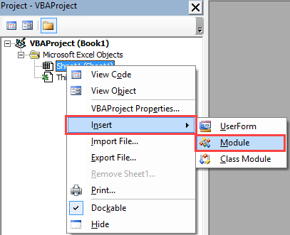
- Copy paste the above code in the module code window.
- Close the VB Editor.
Click here to download the example file.
Now you can use this function as any regular worksheet function in Excel.
CONCATENATE Excel Ranges Using TEXTJOIN Function (available in Excel with Office 365 subscription)
In Excel that comes with Office 365, a new function – TEXTJOIN – was introduced.
This function, as the name suggests, can combine the text from multiple cells into one single cell. It also allows you to specify a delimiter.
Here is the syntax of the function:
TEXTJOIN(delimiter, ignore_empty, text1, [text2], …)
- delimiter – this is where you can specify a delimiter (separator of the text). You can manually enter this or use a cell reference that has a delimiter.
- ignore_empty – if this is TRUE, it will ignore empty cells.
- text1 – this is the text that needs to be joined. It could be a text string, or array of strings, such as a range of cells.
- [text2] – this is an optional argument where you can specify up to 252 arguments that could be text strings or cell ranges.
Here is an example of how the TEXTJOIN function works:

In the above example, a space character is specified as the delimiter, and it combines the text strings in A1:A5.
You can read more about the TEXTJOIN function here.
Have you come across situations where this can be useful? I would love to learn from you. Do leave your footprints in the comments section!
You May Also Like the following Excel tutorials:


54 thoughts on “CONCATENATE Excel Range (with and without separator)”
thank you so much bro!! from the Philippines
For some reason the formula =@CONCATENATEMULTIPLE(A1:A5,” “) OR =CONCATENATEMULTIPLE(A1:A5,” “) in my own spreadsheet. I receive a #NAME error. Only work in your downloadable example – Why would this be happening?
textjoin is awesome
Thank you very much for this tip. As others have said, it solves the =CONCANT issue of time.
I use this daily within Maximo to turn a column of WO #s into a row with a comma and space between each. I then can paste them into a program for modifications.
Textjoin = No more Concatenation torture on many columned joins. Thanks!
Wow this is supremely helpful, saved me A LOT of time! Thanks man.
Your macro just saved my life! Thank you
I. Love. You.
Hy!
Can someone help me with this formula or similiar please?
I want to use texjoin for one row with results only in non empty cells, but I got result with zeroes.
and also I have to combine a column name with data found in particular cell
name1 Name2 Name3
row 0 1 2
=1 Name2, 2 name3
is that possible?
tnx
In case that you have values
Name1 Name2 Name3
0 1 2
in a range A1:C2, than you can insert formula
=IF(A2=0,””,TEXTJOIN(” “,,A2,A1))
into cell A3 and fill it to the right two cells.
Then you will get
(Empty cell),1 Name2, 2 Name3
in cells A3:C3.
Thank you!
Thanks a lot . It worked great. I have 1000s of multiple “|”delimited rows and this function did a great job. God bless you .
Thanks, very helpful! One suggestion is to strip off the number of characters in the separator (accommodates separators with multiple characters, e.g. a comma with a space, like “, “).
CONCATENATEMULTIPLE = Left(Result, Len(Result) – Len(Separator))
This is a more generalized solution to Rowan’s specific empty string (“”) seperator fix. Well done and thanks for sharing.
Note, for some reason in Excel MVBA 7.1, I was unable to apply this code directly. I had to apply the simple math from the second parameter in Len() for the VB editor to accept the code. I.e.:
resLen = Len(Result)
sepLen = Len(Separator)
tmpLen = resLen – sepLen
CONCATENATEMULTIPLE = Left(Result, tmpLen)
Thanks a lot for the code and the explanation. Great function 🙂
Hi, looking for a VBA code to concatenate the complete row like (A1:A25 in A26). what is the easy way to do it…!!
Many thanks for Multiple option – much appreciated
Concatenatemultiple is fantastic! Only limitation I noticed is if you don’t have a separator (using “”) then it cuts off the last value of the text. So with a small if function it was corrected:
If Separator = “” Then
CONCATENATEMULTIPLE = Left(Result, Len(Result))
Else
CONCATENATEMULTIPLE = Left(Result, Len(Result) – 1)
End If
Thanks for providing the fix. I ran into this.
The CONCATENATEMULTIPLE code works well. What about when the number of cells to concatenate is variable? What would this code look like?
Hi,
Does anyone know a way to do the following:
Concatenate the values of several cells into a single cell and separate them with any delimiter of your choosing.
Project Name Result
Project1 Mike Project1, Mike, Neal, Peter
Project1 Neal
Project1 Peter
Project2 Mike Project2, Mike, Neal, Peter
Project2 Neal
Project2 Peter
This could be done much simpler with VBA, but also have many solutions with Excel embedded formulas:
Lets suppose you have the following values in column A:
Project1 Mike
Project1 Neal
Project1 Peter
Project2 Mike
Project2 Neal
Project2 Peter
First, add one row above all and leave it empty, so the content starts with cell A2.
Second, add formula =IF(ROW()=2,LEFT(A2,8)&”, “&RIGHT(A2,LEN(A2)-8-1),IF(LEFT(A2,8)=LEFT(A1,8),B1&”, “&RIGHT(A2,LEN(A2)-8-1),LEFT(A2,8)&”, “&RIGHT(A2,LEN(A2)-8-1))) to cell B2 and fill it down the column B.
For additional clearing add formula =IF(ISNUMBER(FIND(B2,B3)),””,B2) to cell C2 and fill down the column C.
Changing delimiter can be done by changing every “, ” in the first formula.
If your shared word is not “Project1”, you would have to change every 8 (the length of the word Project1) in the first formula with the length of another word.
Thanks, nice little function. Also adapted to use the ‘Len(Separator)’ value:
Function CONCATENATEMULTIPLE(Ref As Range, Separator As String) As String
Dim Cell As Range
Dim Result As String
For Each Cell In Ref
Result = Result & Cell.Value & Separator
Next Cell
CONCATENATEMULTIPLE = Left(Result, Len(Result) – Len(Separator))
End Function
This is a great post and will save me tons of time. Just one query, how would i set up the VBA code to ignore #N/A entries? I want to run the code from a pivot table and the number of results from the pivot changes each time?? Any help would be great. Thanks…..
=IFNA(TEXTJOIN(…..
I think I should clarify my suggestion.
=IFNA(TEXTJOIN(” “,0,$A$1:$A$6),””)
It’s great for getting rid of #N/A if they appear.
There are references on it’s uses on other sites, but it basically is an IF statement that is triggered when #N/A is true, else “”. You can substitute whatever you want to the second part instead of “”. This TEXTJOIN is really useful, and I’ve been using it ever since I stumbled across it.
Perhaps you could implement the TEXTJOIN function from Google Spreadsheet. Here’s my implementation:
Function TEXTJOIN(separator As String, skipEmpty As Boolean, Ref As Range) As String
Dim i As Integer
Dim tmp As String
For Each Cell In Ref
If (Cell.Value “”) Then
tmp = tmp & Cell.Value & separator
End If
Next Cell
TEXTJOIN = Left(tmp, Len(tmp) – Len(separator))
End Function
Thank you for these solutions!
I would have like to alter the VBA method as to avoid empty cells (i.e. so the user can select a whole column, yet concatenate only non-empty cells).
I know it is not trivial – but it would help to make this a more robust function.
Hi,
Does anyone know a way to do the following:
I want to combine or concatenate text in every cell in column A with every cell in column B without repeating or flash fill because that won’t do the trick..
Example here:
COLUMN A contains:
A
B
C
COLUMN B contains:
10
20
30
40
What I want as output in another COLUMN:
A10
A20
A30
A40
B10
B20
B30
B40
C10
C20
C30
C40
Anyone an idea how to do this?
I am looking to do this same thing. Have you figured out how to do this?
One of the solutions without VBA is submitted above.
Another solution without VBA is:
Enter formula =COUNTIF(A:A,”?*”) to cell C1 (counts number of cells with text in column A)
Enter formula =COUNTIF(B:B,”>0″) to cell C2 (counts number of cells with numbers >=0 in column B)
Enter formula =INDIRECT(ADDRESS(QUOTIENT(ROW()-1,$C$2)+1,1)) to cell D1 and fill down until it starts giving zeros.
Enter formula =D1&INDIRECT(ADDRESS(COUNTIF(D$1:D1,D1),2)) to cell E1 and fill down until it has values in column D. Your solution should be in column E.
PS: Formula in cell C1 is given just in need for making pairs with textual data.
Third solution without VBA (in one line) could be done with formula =INDIRECT(ADDRESS(QUOTIENT(ROW()-1,COUNTIF(B:B,”>0″))+1,1))&INDIRECT(IF(MOD(ROW(),COUNTIF(B:B,”>0″))0,ADDRESS(MOD(ROW(),COUNTIF(B:B,”>0″)),2),ADDRESS(COUNTIF(B:B,”>0″),2))) in cell C1 and fill it down until it starts giving superfluous solutions. In case that you are pairing text in column B, change all COUNTIF(B:B,”>0″) in formula with COUNTIF(B:B,”>0”) .
* Correction:
In case that you are pairing text in column B, change all COUNTIF(B:B,”>0″) in formula with COUNTIF(B:B,”?*”) .
Copy values from column A to column C, beginning from C2:C4. Copy values from column B to column D, beginning from D1, but with Paste_Special>>Transpose, so everything start looking as a empty table with letters for rows and numbers for columns. Now select cell D2 and enter formula =$C2&D$1 (dollar signs must be on that places). Now fill in formula till the end of the rows and columns. Now select all 12 values and copy it without moving the selection, then paste>>paste_values. Now you have to place values in one column. Open new sheet, copy 12 values, select B1 and Paste_Special>>Transpose. Now insert formula =IF(ROW()*1/4=INT(ROW()*1/4),ROW()*1/4,INT(ROW()*1/4)+1) into cell A1. The most important thing is number 4, because it is related with number of rows filled wit values. ***In case of 50 rows with data, formula would be =IF(ROW()*1/50=INT(ROW()*1/50),ROW()*1/50,INT(ROW()*1/50)+1).*** Fill down formula (with fours) 12 times (because you have 12 values). Now insert formula =INDIRECT(ADDRESS(ROW()-(A5-1)*4,COLUMN()+(A5-1),4)) in cell B5 and fill down till B12. The most important in this formula is that FIRST number 4 has same role as in previous, and A5 is there because we put formula in B5.***In case of 50 rows with data formula would be =INDIRECT(ADDRESS(ROW()-(A51-1)*50,COLUMN()+(A51-1),4)) *** Number 4 at the end of the formula is relative address and is not related to your number of rows.*** Column B is one of the solutions without using VBA.
Apparently TEXTJOIN is associated with Office 365, NOT Excel 2016.
TEXTJOIN() is NOT available on my desktop version of Excel 2016.
Hey Cornan.. You’re right! I have edited the tutorial accordingly.
Hi Sumit, im in need to of 2018 leave tracker template. Could you share updated excel version to adriana.galiano@gmail.com
Thx for this, perfect replacement for the MCONCAT formula from the now defunct (for anyone on 64bit OS) morefunc add-in
Cool! I was finding for auto update concatenate. Thanks for VBA code.
This is great – thanks!
Would suggest one change to the VBA code – instead of using
CONCATENATEMULTIPLE = Left(Result, Len(Result) – 1), you can use
CONCATENATEMULTIPLE = Left(Result, Len(Result) – Len(Separator)); this will allow for multi-character separators.
… and allows even an empty string as a separator. A nasty little bug 😀
This completely saved my ass today creating contact list spreadsheets to import elsewhere!!!!
Excellent! This did exactly what I needed it to in combination with Dynamic Ranges.
Theres a bug in the code. ExcelConcatenate is not equal to CONCATENATEMULTIPLE you should set CONCATENATEMULTIPLE =
Thanks for sharing such wonder ful trick.
How do you do the reverse, plz suggest.
Hello Alok.. By reverse, you mean to split these words into separate cells? You can do this by using text to column. Have a look at #7 in this – http://trumpexcel.com/2014/08/clean-data-in-excel/
Very Very time saving & Interesting brother, Nice tips
Thanks for commenting.. Glad you liked it 🙂
Can you add sample document?
Thanks…
That is a really cool solution. Will save lots of time. What is the more advanced method that automatically removes the curly brackets?
The more advanced way would be to use two cells. In one cell you would use the F9 key and get the hard coded values, and in another you can have a formula that would automatically remove curly brackets (using replace/substitute). You can go that way if you want this to be partially dynamic. But i would say the one mentioned in the article is easier and faster way.
Very cool. I always had this problem.
Thanks for the comment buddy.. glad it helped 🙂