
Watch Video – Search and Highlight Data Using Conditional Formatting
If you work with large datasets, there can be a need to create a search functionality that allows you to quickly highlight cells/rows for the searched term.
While there is no direct way to do this in Excel, you can create search functionality using Conditional Formatting.
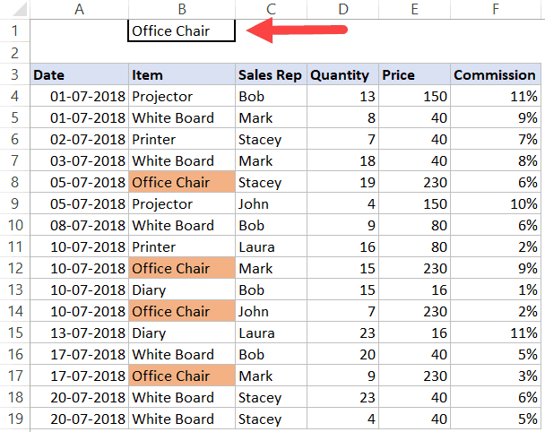
For example, suppose you have a dataset as shown below (in the image). It has columns for Product Name, Sales Rep, and Country.
Now you can use conditional formatting to search for a keyword (by entering it in cell C2) and highlight all the cells that have that keyword.
Something as shown below (where I enter the item name in cell B2 and press Enter, the entire row gets highlighted):
In this tutorial, I will show you how to create this search and highlight functionality in Excel.
Later in the tutorial, we will go a bit advanced and see how to make it dynamic (so that it highlights while you’re typing in the search box).
Click here to download the example file and follow along.
Search and Highlight Matching Cells
In this section. I will show you how to search and highlight only the matching cells in a dataset.
Something as shown below:
Here are the steps to search and highlight all the cells that have the matching text:
- Select the dataset on which you want to apply Conditional Formatting (A4:F19 in this example).
- Click the Home tab.
- In the Styles group, click on Conditional Formatting.
- In the drop-down options, click on New Rule.

- In the ‘New Formatting Rule’ dialog box, click on the option ‘Use a formula to determine which cells to format’.

- Enter the following formula: =A4=$B$1

- Click on ‘Format..’ button.

- Specify the formatting (to highlight cells that match the searched keyword).

- Click OK.
Now type anything in cell B1 and press enter. It will highlight the matching cells in the dataset that contain the keyword in B1.
How does this work?
Conditional Formatting gets applied whenever the formula specified in it returns TRUE.
In the above example, we check each cell using the formula =A4=$B$1
Conditional Formatting checks each cell and verifies it the content in the cell is the same as that in cell B1. If it’s the same, the formula returns TRUE and the cell gets highlighted. If it isn’t the same, the formula returns FALSE and nothing happens.
Click here to download the example file and follow along.
Search and Highlight Rows with Matching Data
If you want to highlight the entire row instead of just the matching cells, you can do that by tweaking the formula a little.
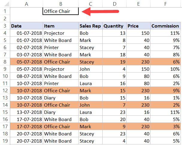
Below is an example where the entire row gets highlighted if the product type matches the one in cell B1.
Here are the steps to search and highlight the entire row:
- Select the dataset on which you want to apply Conditional Formatting (A4:F19 in this example).
- Click the Home tab.
- In the Styles group, click on Conditional Formatting.
- In the drop-down options, click on New Rule.
- In the ‘New Formatting Rule’ dialog box, click on the option ‘Use a formula to determine which cells to format’.
- Enter the following formula: =$B4=$B$1

- Click on ‘Format..’ button.
- Specify the formatting (to highlight cells that match the searched keyword).
- Click OK.
The above steps would search for the specified item in the dataset, and if it finds the matching item, it will highlight the entire row.
Note that this will only check for the item column. If you enter a Sales Rep name here, it will not work. If you want it to work for Sales Rep name, you need to change the formula to =$C4=$B$1
Note: The reason it highlights the entire row and not just the matching cell is that we have used a $ sign before the column reference ($B4). Now when conditional formatting analyzes cells in a row, it checks whether the value in column B of that row is equal to the value in cell B1. So even when it’s analyzing A4 or B4 or C4 and so on, it’s checking for B4 value only (as we have locked column B by using the dollar sign).
You can read more about absolute, relative and mixed references here.
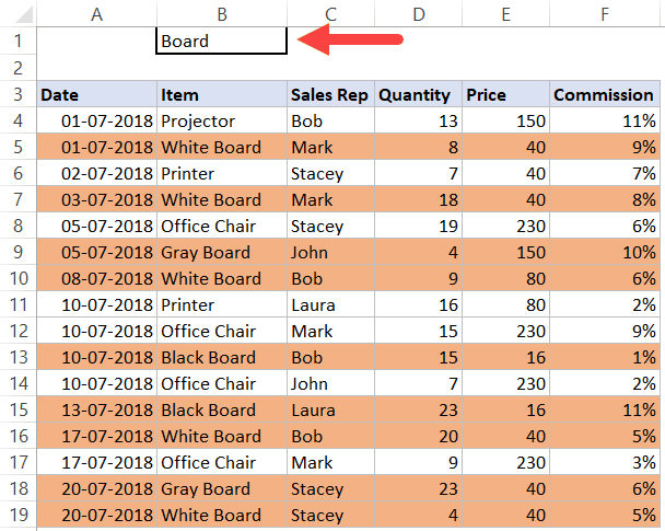
Search and Highlight Rows (based on Partial Match)
In some cases, you may want to highlight rows based on a partial match.
For example, if you have items such as White Board, Green Board, and Gray Board, and you want to highlight all these based on the word Board, then you can do this using the SEARCH function.
Something as shown below:
Here are the steps to do this:
- Select the dataset on which you want to apply Conditional Formatting (A4:F19 in this example).
- Click the Home tab.
- In the Styles group, click on Conditional Formatting.
- In the drop-down options, click on New Rule.
- In the ‘New Formatting Rule’ dialog box, click on the option ‘Use a formula to determine which cells to format’.
- Enter the following formula: =AND($B$1<>””,ISNUMBER(SEARCH($B$1,$B4)))

- Click on ‘Format..’ button.
- Specify the formatting (to highlight cells that match the searched keyword).
- Click OK.
How does this work?
- SEARCH function looks for the search string/keyword in all the cells in a row. It returns an error if the search keyword is not found, and returns a number if it finds a match.
- ISNUMBER function converts the error into FALSE and the numeric values into TRUE.
- AND function checks for an additional condition – that cell C2 should not be empty.
So now, whenever you type a keyword in cell B1 and press Enter, it highlights all the rows that have the cells that contain that keyword.
Bonus Tip: If you want to make the search case sensitive, use the FIND Function instead of SEARCH.
Click here to download the example file and follow along.
Dynamic Search and Highlight Functionality (Highlights as you type)
Using the same Conditional Formatting tricks covered above, you can also take it a step further and make it dynamic.
For example, you can create a search bar where the matching data gets highlighted as you’re typing in the search bar.
Something as shown below:
This can be done using ActiveX controls and can be a good functionality to use when creating reports or dashboards.
Below is a video where I show how to create this:
Did you find this tutorial useful? Let me know your thoughts in the comments section.
You May Also Like the Following Excel Tutorials:


I am trying to do this exact thing but with one added step and I have no idea how. I want to scan into the search box and have the corresponding cell’s column highlighted and remain highlighted until I have completed all scans. After that I want to simply clear the highlight formats and have the original spreadsheet remaining to do it all over again. I am making a really really low key inventory tracking and reordering system that anyone can use. Is this even possible??
Sheet1 column A:A some cells have numbers(suppose 100 numbers).
Sheet2 column A, B C & D having a few numbers (suppose 50 numbers) those exactly match/equal with sheet1numbers.
Now want to highlight cells or rows of sheet1 on the basis of numbers of sheet2.
Tnx to all ecperts in advance.
Wrong explanation.
good lesson
hi! i need help for excel
This formula
=AND($B$1″”,ISNUMBER(SEARCH($B$1,$B4)))
from Search and Highlight Rows (based on Partial Match)
is wrong…
There is a problem with this formular, is all excel have to say about this
Nevermind, replaced , through ; and is now working
I cant get this formula to work. What did you replace=AND($B$1″”,ISNUMBER(SEARCH($B$1,$B4)))
Is there a way to have the highlighted data from search filter to top of dataset? I have a large spreadsheet and have to scroll all the way down to see highlighted rows.
Thanks
HI
I cant get the formula to work. Excel wont recognize it.
I translated to danish.
problem seems to be “”,ELLER
any solution?
=OG($C$2″”,ELLER(ER.TAL(SØG($c$2,$A7:H7,1))))
would apreciate it very much
Nitram
Sorry men. I do not why, in my case, it does not work. In the bets of the scenarios, it highlight like two cells that they do not have anything to do.
Thank you Sumit.
Hello, Why don’t =AND($C$2″”, OR(ISNUMBER(SEARCH($C$2, $B5)))) works?Coz I tried that formula so that even if I just input a string or a keyword, it will highlight that particular word, not the entire row. That formula works but if only I try to input the product, but if i try to input the name and geography it wont work.
Hi Sumit,
I find Search and Highlight Cells using Conditional Formatting very useful however I tried every other possibility to but doesn’t highlight any data. Same applies with Gantt chart as well I could not format the date schedule. I am using Microsoft office 2007. Hope you can help me out.
Hi , I can’t see the necessity here for OR either, i used =SEARCH(input;$B16&$C16&$D16&$E16&$F16) , where $B16 &…. your range for row to be highlited and “input” the name of the cell that searches, also make sure you select the area you want with Shift+Ctrl before you go to Conditional formating, hope it works for you.
I didn’t understand why we have used OR functions here –
=AND($C$2″”,OR($C$2=$B5:$D5))
OR formula would highlight the entire row. The first formula showcases how you can highlight matching cells only (in the countries column). I have used the OR formula in the second tab (in the download file), where the intent is to highlight the entire row.
I understand OR is to highlight the entire row but I did not understand the logic. I mean without OR why it is not working ? -> =AND($C$2″”,$C$2=$B5:$D5)
It doesn’t work without OR as $C$2=$B5:$D5 does not return a single TRUE or FALSE. Rather it returns an array of True/False. If you do not use OR, there would always be FALSE in the array, and hence AND would always return FALSE.
I have a doubt, why C2 is not equal to D5, I mean –> =AND($C$2″”,$C$2=D5) but instead you used =AND($C$2″”,$C$2=B5) which works here.
Can you please explain ?
Hello Deepak.. when we select the entire range (B5:D22) in this case, the formula is applied keeping the active cell in mind. And conditional formatting evaluates each cell based on it. For example, when it is evaluating cell B5, it used the formula =AND($C$2″”,$C$2=B5). When it moves to cell C5, it evaluates it with the formula =AND($C$2″”,$C$2=C5)