
One of the Excel queries I often get is – “How to highlight the Active Row and Column in a data range?”
And I got one last week too.

So I decided to create a tutorial and a video on it. It will save me some time and help the readers too.
Below is a video where I show how to highlight the active row and column in Excel.
In case you prefer written instructions, below is a tutorial with exact steps on how to do it.
Let me first show you what we are trying to achieve.
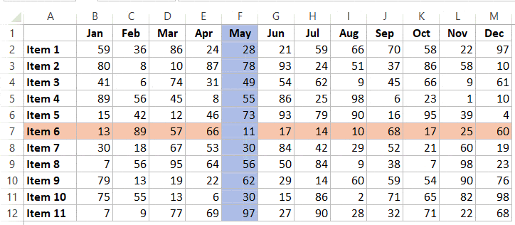
In the above example, as soon as you select a cell, you can see that the row and column also get highlighted. This can be helpful when you’re working with a large dataset and can also be used in Excel Dashboards.
Now let’s see how to create this functionality in Excel.
Highlight the Active Row and Column in Excel
Here are the steps to highlight the active row and column on selection:
- Select the data set in which you to highlight the active row/column.
- Go to the Home tab.
- Click on Conditional Formatting and then click on New Rule.
- In the New Formatting Rule dialog box, select “Use a formula to determine which cells to format”.
- In the Rule Description field, enter the formula: =OR(CELL(“col”)=COLUMN(),CELL(“row”)=ROW())
- Click on the Format button and specify the formatting (the color in which you want the row/column highlighted).
- Click OK.
The above steps have taken care of highlighting the active row and active column (with the same color) whenever there is a selection change event.
However, to make this work, you need to place a simple VBA code in the backend.
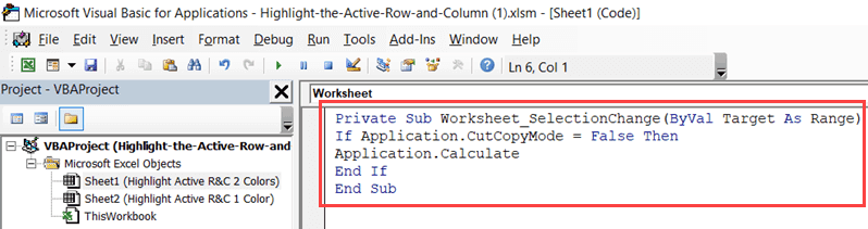
Here is the VBA code that you can copy and paste (exact steps also listed below):
'Code developed by Sumit Bansal from https://trumpexcel.com
Private Sub Worksheet_SelectionChange(ByVal Target As Range)
If Application.CutCopyMode = False Then
Application.Calculate
End If
End Sub
The above VBA code is run whenever there is a selection change in the worksheet. It forces the workbook to recalculate, which then forces the conditional formatting to highlight the active row and the active column.
Normally (without any VBA code), a worksheet refreshes only when there is a change in it (such as data entry or edit).
Also, an IF statement is used in the code to check if the user is trying to copy-paste any data in the sheet.
During copy-paste, the application is not refreshed, and it is allowed.
Here are the steps to copy this VBA code in the backend:
- Go to the Developer tab (can’t find the developer tab? – read this).

- Click on Visual Basic.
- In the VB Editor, on the left, you will see the project explorer that lists all the open workbooks and the worksheets in it. If you can’t see it, use the keyboard shortcut Control + R.

- With your workbook, double-click on the sheet name in which you have the data. In this example, the data is in Sheet 1 and Sheet 2.
- In the code window, copy and paste the above VBA code. You’ll have to copy and paste the code for both sheets if you want this functionality in both sheets.
- Close the VB Editor.
Since the workbook has VBA code in it, save it with a .XLSM extension.
Note that in the steps listed above, the active row and column would get highlighted with the same color. If you want to highlight the active row and column in different colors, use the below formulas:
- =COLUMN()=CELL(“col”)
- =CELL(“row”)=ROW()
In the download file provided with this tutorial, I have created two tabs, one each for single color and dual color highlighting.
Since these are two different formulas, you can specify two different colors.
Useful Notes:
- This method would not impact any formatting/highlighting you have done manually to the cells.
- Conditional formatting is volatile. If you use it on very large datasets, it may lead to a slow workbook.
- The VBA code used above would refresh the workbook every time there is a change in selection.
- CELL Function is available in Excel 2007 and above version for Windows and Excel 2011 and above for Mac. In case you’re using an older version, use this technique by Chandoo.
Want to Level-up your Excel Skills? Consider joining one of my Excel courses:
You May Also Like the Following Excel Tutorials:


Very Good and thank you.
One small issue was that i found copying the formula in it’s BOLD format caused it not to work. I had to re-write it in normal text and it worked fine.
Very good book. Useful for excel beginners
Searching this long grt tutorial and suffer one error also but with someone comment i change according n its work
here he typed:
=OR(CELL(“col”)=COLUMN(),CELL(“row”)=ROW())
everything needs to be caps so:
=OR(CELL(“COL”)=COLUMN(),CELL(“ROW”)=ROW())
thanks for your efforts, but i think Microsoft should add this as a basic excel services , no need to do this long steps
How to enable that please tell me.
Forgot one important thing. I am using Windows 10, 64 bit, Excel office 365.
This is what I wanted. But, it only works on 1 worksheet in my workbook of 10 sheets. I have copied the VBA code on 2 or 3 sheets to see if that works, but still only works on 1 sheet. I would like to be able to not only work on all sheets, but also any other workbook file I need to use it in. Can you help me? Also, is it possible to make this an Excel Add-in, so it would work in any file I open?
I’ve noticed that it’s not possible to use ctrl+z if you make a change in a cell and then selet another cell. Is it possible to Work around this with an additional code of VBA?
Thank you in advance!
Awesome explanation .It helps lot .
Can you post how to work in timing
Ex : 1,1.30,1.0,1.30 ,Sum=5 hrs
If we call calculate in excel it comes =4.60 hrs
Pls support
FIXED:
1. Change to UPPERCASE — (Replace “row” and “col” with “ROW” and “COL”)
2. MANUALLY replace the quotes — (copy paste from browser inserts curly quotes)
jamshaid
can you help me to do this in google sheet ?
thanks
can you help me to do this in google sheet ?
thanks
Guys,
If it does not work for you then in the conditional formating formula delete the quotation marks and type them in again.
Replace below:
=OR(CELL(“col”)=COLUMN(),CELL(“row”)=ROW())
With below:
=OR(CELL(“col”)=COLUMN(),CELL(“row”)=ROW())
If you look closely you see it is a different type of quotation mark: “ ”
Let me know if it worked for you 🙂
It doesn’t work for me 🙁 I need to put ‘ infront of it or my excel doesn’t know what im trying to do or something, is there any solution?
Thanks!
Hi there,
Thanks for the code.
My doubt is code is getting failed when its have background colour applied on the sheet
Doesn’t work
It is not working in my excel
Pure Gold, pure gold. Thank you!
you are just awesome !!! I always wanted to do this !!
Hello,
Is it possible to just highlight the active cell, and not the entire row & column?
In the conditional formatting rules, change =OR(…) to =AND(…)
How to highlight active range in conditional formatting?
sumit
thanks for your effort … it is very helpful.
is one improvement possible – have the highlight work in the middle of cut-paste?
an example …
i am copying data from one person (row) to another person (other row)
when i select row 3, cols b+c, and copy … the proper row and col b highlight.
when i select a cell in row 7 col b to paste, (another person) the highlight does not change (since cutcopymode = false )
until i paste the data into the selected cell , then the highlight changes correctly.
it would be helpful to see the highlight change when i selected the cell – before i paste the data – so i could be sure i had selected the right person/row.
Hi,
Excactly what I need but I type the formula and VBA and it is not working. it is save as .xlsm. Could I send you my file? Thanks for your help
How can I highlight the row depending on a cell entry?
THANK YOU! Your tutorial worked perfectly!
My workbook has multiple sheets. I’m able to follow your instructions and get it to work on the first time. Is there a way to apply this set of instruction for all the sheets? Right now, I’m having to repeat the instructions multiple times for the entire workbook.
Thank you for being so helpful and articulate. It’s people like you who I really appreciate!
What a useful tip! I would love it if I could click over to another workbook without affecting the highlighting. Is there a way to accomplish this?
SOLUTION:
For anyone who tries this and it doesn’t work – as the comment above me mentioned….. RE-TYPE the QUOTATION MARKS ” ” for “col” and “row”. And it should solve the problem.
Thank you!!
Thank yoU!
Thank you!!!
Thanks Boss u r grt since 30 min i m trying n jst i type quotation mark n its worked
thank you!!!!!!
Thank you so much for posting this tutorial. I am a lament user and i was able to follow this tutorial and set up the macro in the developers tab and the conditional formatting in my spreadsheet. It is so much easier to navigate now. You are awesome! Keep doing what you do, it is much appreciated!
Thank you so much for the kind words.. Glad you found the tutorial useful 🙂
Awesome!! Did exactly what I wanted it to do! Thank you!!!
Exactly what I needed except one serious issue: My spreadsheet is CPU intensive. Therefore I’ve turned off auto calculation. This VBA code (as you do note) forces recalculation. Will there be any way around this issue?
Thank you for simple and best explanation given.
Hi Submit, Thanks for your clear & accurate instructions… I had no problems setting this up. Years ago I looked for a Col-Row Highlighter like this but never found it. Today I checked again and found your solution. Great job on both instructions and execution. Thank you!!
You have curly quotes in your example text!! (e.g. “ and ”)
You need normal quotes! (e.g. “)
Otherwise the formulas won’t work if you copy and paste.
Ok well apparently this website automatically formats quotes as curly quotes. So don’t copy anything directly from here. You need to type the quotes into your code manually.
Thanks! Couldn’t figure out why I wasn’t able to get mine to work. 🙂
this formula isn’t working for me! Excel 2016
Hi! How can I activate the undo and redo button?
I had to replace the “,” for a “;” for the formula to work (to be accepted by Excel). Must be a french Excel version whim…
If you’re interested: =OU(CELLULE(“col”)=COLONNE();CELLULE(“row”)=LIGNE())
I, like others, had problems getting this to work, and solved it following the suggestion to type the entire formula by hand into the conditional formatting screen. However, I still had a weird problem. Sometimes when I changed the cell selection, it would not update the highlighting in some of the adjacent blocks and not highlight some of the correct blocks. It seemed to be a screen updating problem on my PC, since scrolling down and back again would fix the problem. Finally, I changed the VBA code to:
Private Sub Worksheet_SelectionChange(ByVal Target As Range)
If Application.CutCopyMode = False Then
Application.ScreenUpdating = “False”
Application.Calculate
Application.ScreenUpdating = “True”
End If
End Sub
to force the screen to update, but I’m not sure why I had to do this.
Thank you!!! Mine wasn’t working at first, but this solved my problem!
HI, I followed these tips exactly. But it does not work. I think my conditional formatting may be the issue. I have had similar challenges using CF in the past.
This worked great for me. Just what I needed. Thank you!
For spanish people:
=O(CELDA(“columna”)=COLUMNA();CELDA(“fila”)=FILA())
Nice of course, but a little more should be told.
A little more efforts are needed if you intend to use it for highlighting different rows/columns in multiple workbooks/worksheets.
The CELL function works on “Application level” – it provides information for the currently active cell (regardless of worksheet or workbook).
For example if you apply this trick to sheet1 in workbook A, and then you edit cell C3 in workbook B row 3 and column C in workbook A sheet1 will be highlighted. Of course situations exist when this may be exactly what one needs.
I thought it is good to mention this.
I followed all the steps but no highlight is seen.
Not sure what I’m doing wrong.
The example file works for me even though it popped up an VB error, oddly only the 1st time when I opened it.
I downloaded the excel example (and from what I can tell) – everything is the same. It’s still not working. I assume since saving as a .XLSM extension is not an option it’s set as a default??
Never mind – I read other comments and typed in everything manually. Works like a charm!!
Also, when typing in the conditional formatting code use ALL CAPS. 🙂
Thank you for this!!
Thanks for sharing this. I only have a problem when i’m using 2 excel windows side by side. Because when I swicht to the other window the cell formating in the first window changes. I there any solution for this?
Hi, it is not working for me, I have Office 365 and have enabled the macros copying all the details but nothing gets highlighted. Any idea what I’m doing wrong?
Doesn’t work for me. VBA code is identical, conditional formatting is identical. It’s Excel 2016. Any suggestions?
Hi,
Is there a way to make this work with a dynamic selection ? I would like this to work after I paste in a new set of data/selection (The selection will have the same columns, but the rows varies.
Thanks
=OR(CELL(“COL”)=COLUMN(),CELL(“ROW”)=ROW()) worked for me instead of =OR(CELL(“col”)=COLUMN(),CELL(“row”)=ROW())
Hi, I loved this highlight, but I need to keep using the “COPY” and “PAST” function as numbers and formulas. It is possible?
You can use the following VBA code:
Private Sub Worksheet_SelectionChange(ByVal Target As Range)
If Application.CutCopyMode = False Then
Application.Calculate
End If
End Sub
How to do the trick with Mac? Because I just keep getting message: Variable uses an Automation type not supported in Visual Basic. And I can’t go around it.
Hi Sumit,
I am trying to use my spreadsheet with your modification. A problem I have found is that although I can copy a range of cells which are highlighted as normal, the paste function is greyed out. Ctrl+V also doesn’t work. Any ideas why?
Me again,
Maybe I should have read the instructions more carefully!! ;-)) I missed out the VBA code. Added it and now working brilliantly.
Hi again, Just discovered that it works if I just select a cell and then press either page up or page down.
Hi Sumit, I have tried to introduce this trick into a spreadsheet using Excel 2016. I used the conditional format method without the macro. Is it necessary to write the macro as well? The only way I can get it to work is to select a cell, press F2, and then press enter. In your example it is not necessary to go the F2 then enter route. Is there an option setting I am missing? Something to do with automatic screen updating?
General Copy and Past not working
is there a way to fix it? and make genera copy and paste work?
Use the following VBA code:
Private Sub Worksheet_SelectionChange(ByVal Target As Range)
If Application.CutCopyMode = False Then
Application.Calculate
End If
End Sub
Like the tip very much. but it is not working for me. i am using office 2010.
cells remain without highlight. cannot make out what’s wrong.
Hey Sunil, Did you copy the formula as is? I noticed that the quotation marks get copied in a different format. Try entering the formula manually and it should work
great. after few hits and trial it worked. now to replicate it in all my worksheets??? any shortcuts or just copy the conditional formatting and vba to the other sheets.
Thanks for the help – greatly appreciated.
Hi Sumit, is there any way to apply this to all worksheets in a workbook? Also, how to make it easily applicable to a new workbook?
thanks
Thanks – had to type it out myself (the quotations were the issue), works like a charm on my huge spreadsheets.
Nice trick
to the VBA i have added some lines.
With Application
.ScreenUpdating = False
.EnableEvents = False
.Calculate
.ScreenUpdating = True
.EnableEvents = True
End With
screenupdating will help speeding up the highlighting
enableevents will prevent the triggering Worksheet_Change
Thanks for sharing Miaousse 🙂 It sure will make the code better
Hi – that’s great – can you give the revised vba code please, as I’m not sure if this is an add-on to the one you gave earlier. thanks
Where do you add those lines?