
Excel has a lot of functions – about 450+ of them.
And many of these are simply awesome. The amount of work you can get done with a few formulas still surprises me (even after having used Excel for 10+ years).
And among all these amazing functions, the INDEX MATCH functions combo stands out.
I am a huge fan of INDEX MATCH combo and I have made it pretty clear many times.
I even wrote an article about Index Match Vs VLOOKUP which sparked a little bit of debate (you can check the comments section for some firework).
And today, I am writing this article solely focussed on Index Match to show you some simple and advanced scenarios where you can use this powerful formula combo and get the work done.
Note: There are other lookup formulas in Excel – such as VLOOKUP and HLOOKUP and these are great. Many people find VLOOKUP to be easier to use (and that’s true as well). I believe INDEX MATCH is a better option in many cases. But since people find it difficult, it gets used less. So I am trying to simplify it using this tutorial.
Now before I show you how the combination of INDEX MATCH is changing the world of analysts and data scientists, let me first introduce you to the individual parts – INDEX and MATCH functions.
INDEX Function: Finds the Value-Based on Coordinates
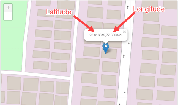
The easiest way to understand how Index function works is by thinking of it as a GPS satellite.
As soon as you tell the satellite the latitude and longitude coordinates, it will know exactly where to go and find that location.
So despite having a mind-boggling number of lat-long combinations, the satellite would know exactly where to look.
I quickly did a search for my work location and this is what I got.
Anyway, enough of geography.
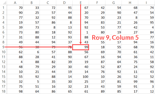
Just like a satellite needs latitude and longitude coordinates, the INDEX function in Excel would need the row and column number to know what cell you’re referring to.
And that’s Excel INDEX function in a nut-shell.
So let me define it in simple words for you.
The INDEX function will use the row number and column number to find a cell in the given range and return the value in it.
All by itself, INDEX is a very simple function, with no utility. After all, in most cases, you are not likely to know the row and column numbers.
But…
The fact that you can use it with other functions (hint: MATCH) that can find the row number and the column number makes INDEX an extremely powerful Excel function.
Below is the syntax of the INDEX function:
=INDEX (array, row_num, [col_num])
=INDEX (array, row_num, [col_num], [area_num])
- array – a range of cells or an array constant.
- row_num – the row number from which the value is to be fetched.
- [col_num] – the column number from which the value is to be fetched. Although this is an optional argument, but if row_num is not provided, it needs to be given.
- [area_num] – (Optional) If array argument is made up of multiple ranges, this number would be used to select the reference from all the ranges.
INDEX function has 2 syntaxes (just FYI).
The first one is used in most cases. The second one is used in advanced cases only (such as doing a three-way lookup) which we will cover in one of the examples later in this tutorial.
But if you’re new to this function, just remember the first syntax.
Below is a video that explains how to use the INDEX function
MATCH Function: Finds the Position baed on a Lookup Value
Going back to my previous example of longitude and latitude, MATCH is the function that can find these positions (in the Excel spreadsheet world).
In simple language, the Excel MATCH function can find the position of a cell in a range.
And on what basis would it find a cell’s position?
Based on the lookup value.
For example, if you have a list as shown below and you want to find the position of the name ‘Mark’ in it, then you can use the MATCH function.
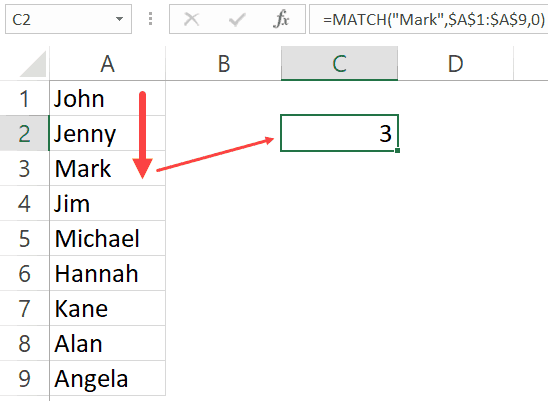
The function returns 3, as that’s the position of the cell with the name Mark in it.
MATCH function starts looking from top to bottom for the lookup value (which is ‘Mark’) in the specified range (which is A1:A9 in this example). As soon as it finds the name, it returns the position in that specific range.
Below is the syntax of the MATCH function in Excel.
=MATCH(lookup_value, lookup_array, [match_type])
- lookup_value – The value for which you are looking for a match in the lookup_array.
- lookup_array – The range of cells in which you are searching for the lookup_value.
- [match_type] – (Optional) This specifies how excel should look for a matching value. It can take three values -1, 0 , or 1.
Understanding Match Type Argument in MATCH Function
There is one additional thing you need to know about the MATCH function, and it’s about how it goes through the data and finds the cell position.
The third argument of the MATCH function can be 0, 1 or -1.
Below is an explanation of how these arguments work:
- 0 – this will look for an exact match of the value. If an exact match is found, the MATCH function will return the cell position. Else, it will return an error.
- 1 – this finds the largest value that is less than or equal to the lookup value. For this to work, your data range needs to be sorted in ascending order.
- -1 – this finds the smallest value that is greater than or equal to the lookup value. For this to work, your data range needs to be sorted in descending order.
Below is a video that explains how to use the MATCH function (along with the match type argument)
To summarize and put it in simple words:
- INDEX needs the cell position (row and column number) and gives the cell value.
- MATCH finds the position by using a lookup value.
Let’s Combine Them to Create a Powerhouse (INDEX + MATCH)
Now that you have a basic understanding of how INDEX and MATCH functions work individually, let’s combine these two and learn about all the wonderful things it can do.
To understand this better, I have a few examples that use the INDEX MATCH combination.
I will start with a simple example and then show you some advanced use cases as well.
Click here to download the example file
Example 1: A simple Lookup Using INDEX MATCH Combo
Let’s do a simple lookup with INDEX/MATCH.
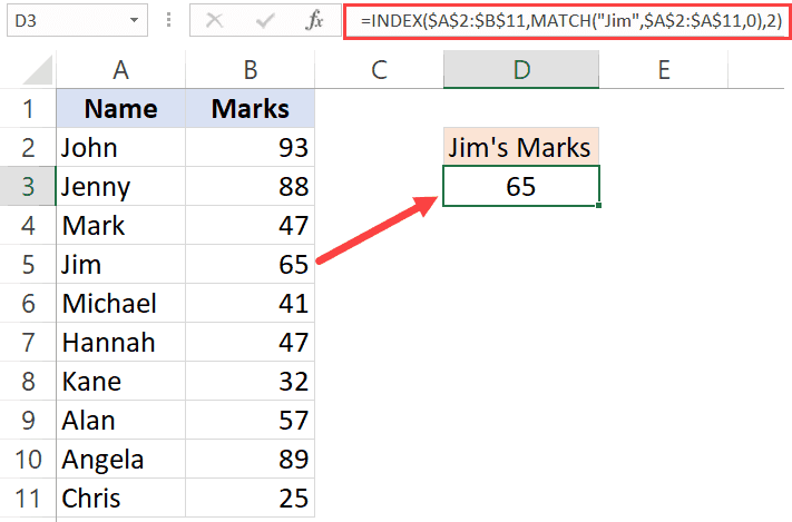
Below is a table where I have the marks for ten students.
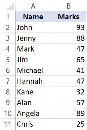
From this table, I want to find the marks for Jim.
Below is the formula that can easily do this:
=INDEX($A$2:$B$11,MATCH("Jim",$A$2:$A$11,0),2)
Now, if you’re thinking this can easily be done using a VLOOKUP function, you’re right! This is not the best use of INDEX MATCH awesomeness. Despite the fact that I am a fan of INDEX MATCH, it is a little more difficult than VLOOKUP. If fetching data from a column on the right is all you want to do, I recommend you use VLOOKUP.
The reason I have shown this example, which can also easily be done with VLOOKUP is to show you how INDEX MATCH works in a simple setting.
Now let me show a benefit of INDEX MATCH.
Suppose you have the same data, but instead of having it in columns, you have it in rows (as shown below).

You know what, you can still use INDEX MATCH combo to get Jim’s marks.
Below is the formula that will give you the result:
=INDEX($B$1:$K$2,2,MATCH(“Jim”,$B$1:$K$1,0))
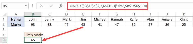
Note that you need to change the range and switch the row/column parts to make this formula work for horizontal data as well.
This can’t be done with VLOOKUP, but you can still do this easily with HLOOKUP.
INDEX MATCH combination can easily handle horizontal as well as vertical data.
Click here to download the example file
Example 2: Lookup to the Left
It’s more common than you think.
A lot of times, you may be required to fetch the data from a column which is to the left of the column that has the lookup value.
Something as shown below:
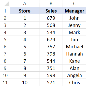
To find out Michael’s sales, you will have to do a lookup on the left.
If you’re thinking VLOOKUP, let me stop your right there.
VLOOKUP is not made to look for and fetch the values on the left.
Can you still do it using VLOOKUP?
Yes, you can!
But that can turn into a long and ugly formula.
So if you want to do a lookup and fetch data from the columns on the left, you are better off using INDEX MATCH combo.
Below is the formula that will get Michael’s sales number:
=INDEX($A$2:$C$11,MATCH("Michael",C2:C11,0),2)
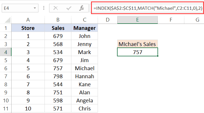
Another point here for INDEX MATCH. VLOOKUP can fetch the data only from the columns that are to the right of the column that has the lookup value.
Example 3: Two Way Lookup
So far, we have seen the examples where we wanted to fetch the data from the column adjacent to the column that has the lookup value.
But in real life, the data often spans through multiple columns.
INDEX MATCH can easily handle a two-way lookup.
Below is a dataset of the student’s marks in three different subjects.
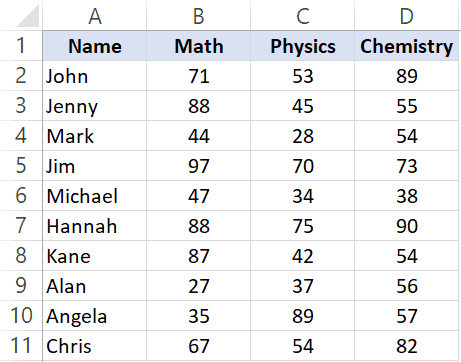
If you want to quickly fetch the marks of a student in all three subjects, you can do that with INDEX MATCH.
The below formula will give you the marks for Jim for all the three subjects (copy and paste in one cell and drag to fill other cells or copy and paste on other cells).
=INDEX($B$2:$D$11,MATCH($F$3,$A$2:$A$11,0),MATCH(G$2,$B$1:$D$1,0))

Let me quickly also explain this formula.
INDEX formula uses B2:D11 as the range.
The first MATCH uses the name (Jim in cell F3) and fetches the position of it in the names column (A2:A11). This becomes the row number from which the data needs to be fetched.
The second MATCH formula uses the subject name (in cell G2) to get the position of that specific subject name in B1:D1. For example, Math is 1, Physics is 2 and Chemistry is 3.
Since these MATCH positions are fed into the INDEX function, it returns the score based on the student name and subject name.
This formula is dynamic, which means that if you change the student name or the subject names, it would still work and fetch the correct data.
One great thing about using INDEX/MATCH is that even if you interchange the names of the subjects, it will continue to give you the correct result.
Example 4: Lookup Value From Multiple Column/Criteria
Suppose you have a dataset as shown below and you want to fetch the marks for ‘Mark Long’.

Since the data is in two columns, I can’t a lookup for Mark and get the data.
If I do it that way, I am going to get the marks data for Mark Frost and not Mark Long (because the MATCH function will give me the result for the MARK it meets).
One way of doing this is to create a helper column and combine the names. Once you have the helper column, you can use VLOOKUP and get the marks data.
If you’re interested in learning how to do this, read this tutorial on using VLOOKUP with multiple criteria.
But with INDEX/MATCH combo, you don’t need a helper column. You can create a formula that handles multiple criteria in the formula itself.
The below formula will give the result.
=INDEX($C$2:$C$11,MATCH($E$3&"|"&$F$3,$A$2:A11&"|"&$B$2:$B$11,0))

Let me quickly explain what this formula does.
The MATCH part of the formula combines the lookup value (Mark and Long) as well as the entire lookup array. When $A$2:A11&”|”&$B$2:$B$11 is used as the lookup array, it actually checks the lookup value against the combined string of first and last name (separated by the pipe symbol).
This ensures that you get the right result without using any helper columns.
You can do this kind of lookup (where there are multiple columns/criteria) with VLOOKUP as well, but you need to use a helper column. INDEX MATCH combo makes it slightly easy to do this without any helper columns.
Example 5: Get Values from Entire Row/Column
In the examples above, we have used the INDEX function to get value from a specific cell. You provide the row and column number, and it returns the value in that specific cell.
But you can do more.
You can also use the INDEX function to get the values from an entire row or column.
And how can this be useful you ask!
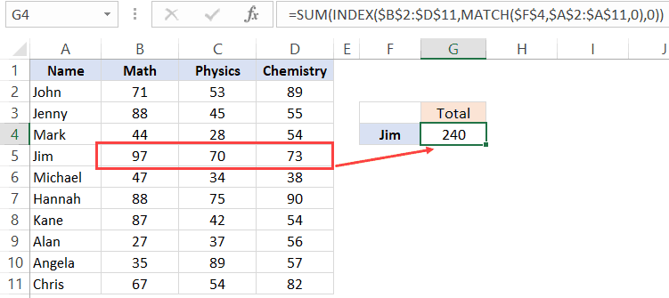
Suppose you want to know the total score of Jim in all the three subjects.
You can use the INDEX function to first get all the marks of Jim and then use the SUM function to get a total.
Let’s see how to do this.
Below I have the scores of all the students in three subjects.
The below formula will give me the total score of Jim in all the three subjects.
=SUM(INDEX($B$2:$D$11,MATCH($F$4,$A$2:$A$11,0),0))
Let me explain how this formula works.
The trick here is to use 0 as the column number.
When you use 0 as the column number in the INDEX function, it will return all the row values. Similarly, if you use 0 as the row number, it will return all the values in the column.
So the below part of the formula returns an array of values – {97, 70, 73}
INDEX($B$2:$D$11,MATCH($F$4,$A$2:$A$11,0),0)
If you just enter this above formula in a cell in Excel and hit enter, you will see a #VALUE! error. This is because it’s not returning a single value, but an array of value.
But don’t worry, the array of values are still there. You can check this by selecting the formula and press the F9 key. It will show you the result of the formula which in this case is an array of three value – {97, 70, 73}
Now, if you wrap this INDEX formula in the SUM function, it will give you the sum of all the marks scored by Jim.
You can also use the same to get the highest, lowest and average marks of Jim.
Just like we have done this for a student, you can also do this for a subject. For example, if you want the average score in a subject, you can keep the row number as 0 in the INDEX formula and it will give you all the column values of that subject.
Click here to download the example file
Example 6: Find the Student’s Grade (Approximate Match Technique)
So far, we have used the MATCH formula to get the exact match of the lookup value.
But you can also use it to do an approximate match.
Now, what the hell is Approximate Match?
Let me explain.
When you’re looking for stuff such as names or ids, you’re looking for an exact match. But sometimes, you need to know the range in which your lookup values lie. This is usually the case with numbers.
For example, as a class teacher, you may want to know what’s the grade of each student in a subject, and the grade is decided based on the score.
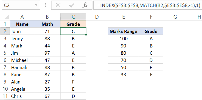
Below is an example, where I want the grade for all the students and the grading is decided based on the table on the right.
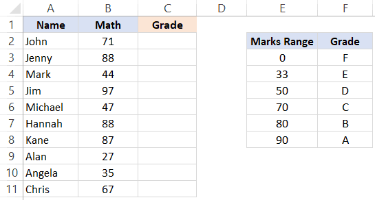
So if a student gets less than 33, the grade is F and if he/she gets less than 50 but more than 33, it’s E, and so on.
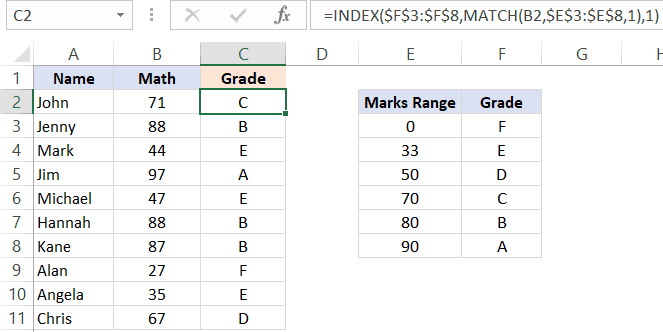
Below is the formula that will do this.
=INDEX($F$3:$F$8,MATCH(B2,$E$3:$E$8,1),1)
Let me explain how this formula works.
In the MATCH function, we have used 1 as the [match_type] argument. This argument will return the largest value that is less than or equal to the lookup value.
This means that the MATCH formula goes through the marks range, and as soon as it finds a marks range that is equal to or less than the lookup marks value, it will stop there and return its position.
So if the lookup mark value is 20, the MATCH function would return 1 and if it’s 85, it would return 5.
And the INDEX function uses this position value to get the grade.
IMPORTANT: For this to work, your data needs to be sorted in ascending order. If it’s not, you can get wrong results.
Note that the above can also be done using below VLOOKUP formula:
=VLOOKUP(B2,$E$3:$F$8,2,TRUE)
But MATCH function can go a step further when it comes to approximate match.
You can also have a descending data and can use INDEX MATCH combo to find the result. For example, if I change the order of the grade table (as shown below), I can still find the grades of the students.
To do this, all I have to do is change the [match_type] argument to -1.
Below is the formula that I have used:
=INDEX($F$3:$F$8,MATCH(B2,$E$3:$E$8,-1),1)
VLOOKUP can also do an approximate match but only when data is sorted in ascending order(but it doesn’t work if the data is sorted in descending order).
Example 7: Case Sensitive Lookups
So far all the lookups we have done have been case insensitive.
This means that whether the lookup value was Jim or JIM or jim, it didn’t matter. You’ll get the same result.
But what if you want the lookup to be case sensitive.
This is usually the case when you have large data sets and a possibility of repetition or distinct names/ids (with the only difference being the case)
For example, suppose I have the following data set of students where there are two students with the name Jim (the only difference being that one is entered as Jim and another one as jim).

Note that there are two students with the same name – Jim (cell A2 and A5).
Since a normal lookup wouldn’t work, you need to do a case sensitive lookup.
Below is the formula that will give you the right result. Since this is an array formula, you need to use Control + Shift + Enter.
=INDEX($B$2:$B$11,MATCH(TRUE,EXACT(D3,A2:A11),0),1)

Let me explain how this formula works.
The EXACT function checks for an exact match of the lookup value (which is ‘jim’ in this case). It goes through all the names and returns FALSE if it isn’t a match and TRUE if it’s a match.
So the output of the EXACT function in this example is – {FALSE;FALSE;FALSE;TRUE;FALSE;FALSE;FALSE;FALSE;FALSE;FALSE}
Note that there is only one TRUE, which is when the EXACT function found a perfect match.
The MATCH function then finds the position of TRUE in the array returned by the EXACT function, which is 4 in this example.
Once we have the position, the INDEX function uses it to find the marks.
Example 8: Find the Closest Match
Let’s get a little advanced now.
Suppose you have a dataset where you want to find the person who has the work experience closest to the required experience (mentioned in cell D2).
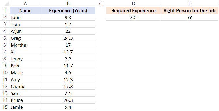
While lookup formulas are not made to do this, you can combine it with other functions (such as MIN and ABS) to get this done.
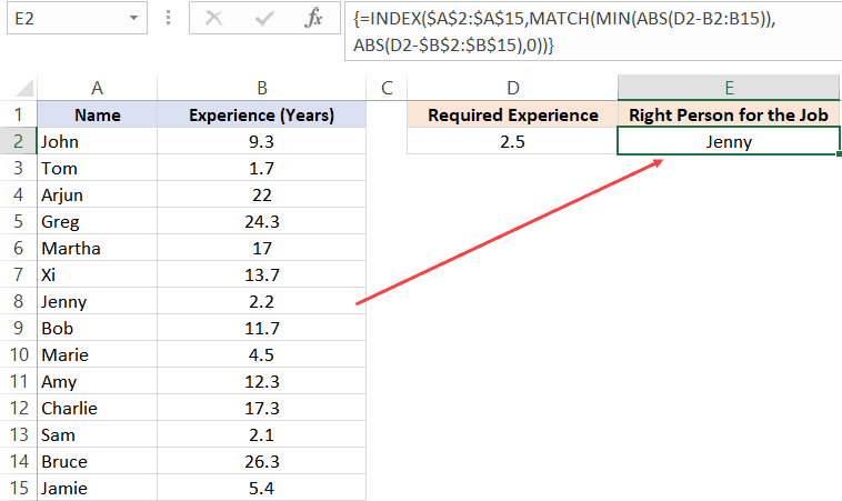
Below is the formula that will find the person with the experience closest to the required one and return the name of the person. Note that the experience needs to be closest (which can be either less or more).
=INDEX($A$2:$A$15,MATCH(MIN(ABS(D2-B2:B15)),ABS(D2-$B$2:$B$15),0))
Since this is an array formula, you need to use Control + Shift + Enter.
The trick in this formula is to change the lookup value and lookup array to find the minimum experience difference in required and actual values.
Before I explain the formula, let’s understand how you would do it manually.
You will go through each cell in column B and find the difference in the experience between what is required and the one that a person has. Once you have all the differences, you will find the one which is minimum and fetch the name of that person.
This is exactly what we are doing with this formula.
Let me explain.
The lookup value in the MATCH formula is MIN(ABS(D2-B2:B15)).
This part gives you the minimum difference between the given experience (which is 2.5 years) and all the other experiences. In this example, it returns 0.3
Note that I have used ABS to make sure I am looking for the closest (which can be more or less than the given experience).
Now, this minimum value becomes our lookup value.
The lookup array in the MATCH function is ABS(D2-$B$2:$B$15).
This gives us an array of numbers from which 2.5 (the required experience) has been subtracted.
So now we have a lookup value (0.3) and a lookup array ({6.8;0.8;19.5;21.8;14.5;11.2;0.3;9.2;2;9.8;14.8;0.4;23.8;2.9})
MATCH function finds the position of 0.3 in this array, which is also the position of the person’s name who has the closest experience.
This position number is then used by the INDEX function to return the name of the person.
Related Read: Find the Closest Match in Excel (examples using lookup formulas)
Click here to download the example file
Example 9: Use INDEX MATCH with Wildcard Characters
If you want to look up a value when there is a partial match, then you need to use wildcard characters.
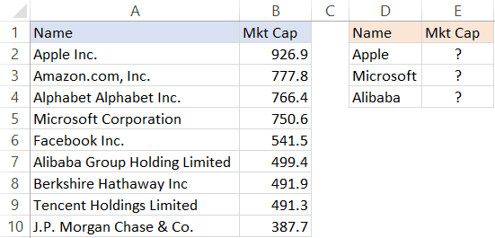
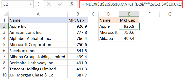
For example, below is a dataset of company name and their market capitalizations and you want to want to get the market cap. data for the three companies on the right.
Since these are not exact matches, you can’t do a regular lookup in this case.
But you can still get the right data by using an asterisk (*), which is a wildcard character.
Below is the formula that will give you the data by matching the company names from the main column and fetching the market cap figure for it.
=INDEX($B$2:$B$10,MATCH(D2&”*”,$A$2:$A$10,0),1)
Let me explain how this formula works.
Since there is no exact match of lookup values, I have used D2&”*” as the lookup value in the MATCH function.
An asterisk is a wildcard character that represents any number of characters. This means that Apple* in the formula would mean any text string that starts with the word Apple and can have any number of characters after it.
So when Apple* is used as the lookup value and the MATCH formula looks for it in column A, it returns the position of ‘Apple Inc.’, as it starts with the word Apple.
You can also use wildcard characters to find text strings where the lookup value is in between. For example, if you use *Apple* as the lookup value, it will find any string that has the word apple anywhere in it.
Note: This technique works well when you only have one instance of matching. But if you have multiple instances of matching (for example Apple Inc and Apple Corporation, then the MATCH function would return the position of the first matching instance only.
Example 10: Three Way Lookup
This is an advanced use of INDEX MATCH, but I will still cover it to show you the power of this combination.
Remember I said that INDEX function has two syntaxes:
=INDEX (array, row_num, [col_num])
=INDEX (array, row_num, [col_num], [area_num])
So far in all our examples, we have only used the first one.
But for a three-way lookup, you need to use the second syntax.
Let me first explain what a three-way look means.
In a two-way lookup, we use the INDEX MATCH formula to get the marks when we have the student’s name and the subject name. For example, fetching the marks of Jim in Math is a two-way lookup.
A three-way look would add another dimension to it. For example, suppose you have a dataset as shown below and you want to know the score of Jim in Math in Mid-term exam, then this would be three-way lookup.
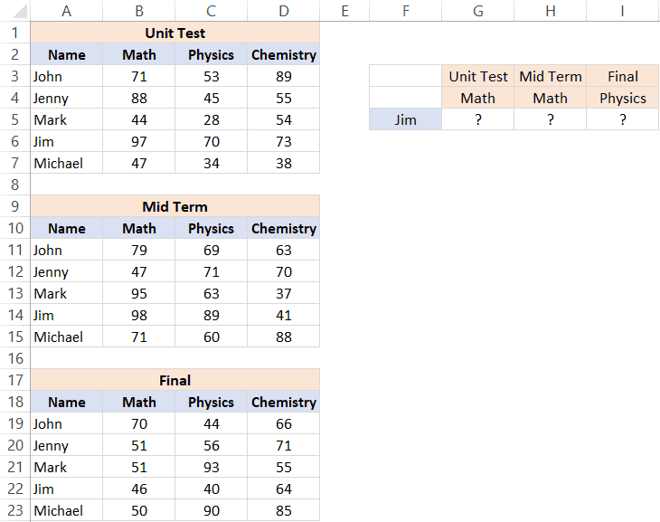
Below is the formula that will give the result.
=INDEX(($B$3:$D$7,$B$11:$D$15,$B$19:$D$23),MATCH($F$5,$A$3:$A$7,0),MATCH(G$4,$B$2:$D$2,0),(IF(G$3="Unit Test",1,IF(G$3="Mid Term",2,3))))
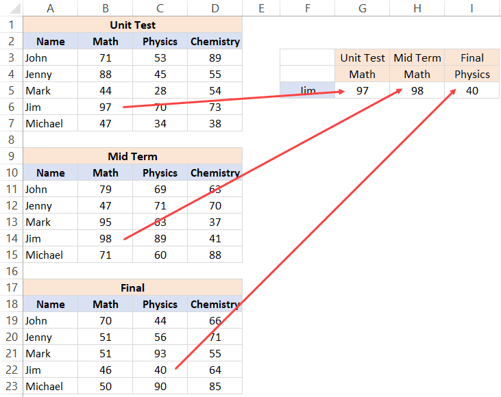
The above formula checked for three things – the name of the student, the subject, and the exam. After it finds the right value, it returns it in the cell.
Let me explain how this formula works by breaking down the formula into parts.
- array – ($B$3:$D$7,$B$11:$D$15,$B$19:$D$23): Instead of using a single array, in this case, I have used three arrays within parenthesis.
- row_num – MATCH($F$5,$A$3:$A$7,0): MATCH function is used to find the position of the student’s name in cell $F$5 in the list of student’s name.
- col_num – MATCH(G$4,$B$2:$D$2,0): MATCH function is used to find the position of the subject name in cell $B$2 in the list of subject’s name.
- [area_num] – IF(G$3=”Unit Test”,1,IF(G$3=”Mid Term”,2,3)): The area number value tells the INDEX function which of the three arrays to use to fetch the value. If the exam is Unit Term, the IF function would return 1 and the INDEX function would use the first array to fetch the value. If the exam is Mid-term, the IF formula would return 2, else it will return 3.
This is an advanced example of using INDEX MATCH, and you’re unlikely to find a situation when you have to use this. But it’s still good to know what Excel formulas can do.
Click here to download the example file
Why is INDEX/MATCH Better than VLOOKUP?
OR Is it?
Yes, it is – in most cases.
I will present my case in a while.
But before I do that, let me say this – VLOOKUP is an extremely useful function and I love it. It can do a lot of things in Excel and I use it every now and then myself. Having said that, it doesn’t mean that there can’t be anything better, and INDEX/MATCH (with more flexibility and functionalities) is better.
So if you want to do some basic lookup, you’re better off using VLOOKUP.
INDEX/MATCH is VLOOKUP on steroids. And once you learn INDEX/MATCH, you might always prefer using it (especially because of the flexibility it has).
Without stretching it too far, let me quickly give you the reasons why INDEX/MATCH is better than VLOOKUP.
INDEX/MATCH can look to the Left (as well as to the right) of the lookup value
I covered it in one of the example above.
If you have a value which is on the left of the lookup value, you can’t do that with VLOOKUP
At least not with just VLOOKUP.
Yes, you can combine VLOOKUP with other formulas and get it done, but it gets complicated and messy.
INDEX/MATCH, on the other hand, is made to lookup everywhere (be it left, right, up, or down)
INDEX/MATCH can work with vertical and horizontal ranges
Again, with full respect to VLOOKUP, it’s not made to do this.
After all, the V in VLOOKUP stands for vertical.
VLOOKUP can only go through data that is vertical, while INDEX/MATCH can go through data vertically as well horizontally.
Of course, there is the HLOOKUP function to take care of horizontal lookup, but it isn’t VLOOKUP then.. right?
I like the fact that INDEX MATCH combo is flexible enough to work with both vertical and horizontal data.
VLOOKUP cannot work with descending data
When it comes to the approximate match, VLOOKUP and INDEX/MATCH are at the same level.
But INDEX MATCH takes the point as it can also handle data that is in descending order.
I show this in one of the examples in this tutorial where we have to find the grade of students based on the grading table. If the table is sorted in descending order, VLOOKUP would not work (but INDEX MATCH would).
INDEX/MATCH can be slightly faster
I will be truthful. I didn’t run this test myself.
I am relying on the wisdom an Excel master – Charley Kyd.
The difference in speed in VLOOKUP and INDEX/MATCH is hardly noticeable when you have small data sets. But if you have thousands of rows and many columns, this can be a deciding factor.
In his article, Charley Kyd states:
“At its worst, the INDEX-MATCH method is about as fast as VLOOKUP; at its best, it’s much faster.”
INDEX/MATCH is Independent of the Actual Column Position
If you have a dataset as shown below as you’re fetching the score of Jim in Physics, you can do that using VLOOKUP.
And to do that, you can specify the column number as 3 in VLOOKUP.
All is fine.
But what if I delete the Math column.
In that case, the VLOOKUP formula will break.
Why? – Because it was hardcoded to use the third column, and when I delete a column in between, the third column becomes the second column.
Using INDEX/MATCH, in this case, is better as you can make the column number dynamic by using MATCH. So instead of a column number, it checks for the subject name and uses that to return the column number.
Surely you can do that by combining VLOOKUP with MATCH, but if you combining anyway, why not do it with INDEX which is a lot more flexible.
When using INDEX/MATCH, you can safely insert/delete columns in your dataset.
Despite all these factors, there is a reason VLOOKUP is so popular.
And it’s a big reason.
VLOOKUP is easier to use
VLOOKUP only takes a maximum of four arguments. If you can wrap your head around these four, you’re good to go.
And since most of the basic lookup cases are handled by VLOOKUP as well, it has quickly become the most popular Excel function.
I call it the King of Excel functions.
INDEX/MATCH, on the other hand, is a little more difficult to use. You may get a hang if it when you start using it, but for a beginner, VLOOKUP is far more easy to explain and learn.
And this is not a zero-sum game.
So, if you’re new to the lookup world and don’t know how to use VLOOKUP, better learn that.
I have a detailed guide on using VLOOKUP in Excel (with lots of examples)
My intent in this article is not to pitch two awesome functions against each other. I wanted to show you the power of INDEX MATCH combo and all the great things it can do.
Hope you found this article useful.
Let me know your thoughts in the comments section, and in case you find any mistake in this tutorial, please let me know.
You May Also Like the Following Excel Tutorials:


Example 4: Merging of Range is not working properly in Office 365. Any work around to work properly.
Thank God that I found this blog. Super helpful. you have helped me to save ~4 hrs effort of month end work. thanks a ton
Thank you, all the examples are very clear.
Perfect!! Very useful, Thanks a lot.
very useful and easy to understand. thank you…
Perfect material love it !!!
i use this formula and it is very useful thanks a lot.
How do you do this partial match when you are pulling the data from another worksheet?
Hi sir , if John is in a1,a5,a8 how we will data from b from respective row , I tried using index but it end with showing results of b1 only
Hi Sir, Your Formula is not working of required field
Please Explain it.
Example 10: Three Way Lookup
=INDEX(($B$3:$D$7,$B$11:$D$15,$B$19:$D$23),MATCH($F$5,$A$3:$A$7,0),MATCH(G$4,$B$2:$D$2,0),(IF(G$3=”Unit Test”,1,IF(G$3=”Mid Term”,2,3))))
would the free info be downloadable? also, trying to find the pipe symbol? Thank You
Hey Sumit thanks for all the great info. Im hoping you can help me with something that I’ve been trying to figure out for DAYS!!! I think index match is what I need but still can’t get it to work.
Im tracking economic data and trying to sort it by the day of week. I want to split it into weekdays, monday – friday. However, some data comes out on Sunday so what I want to do is group all data that came out from 4pm sunday to 4pm monday and put it into Monday’s cell. Likewise the data that comes out 4pm monday to 4pm tuesday will get into tuesdays cell.
The way I have it arranged is: weekday(), hour(), data (Column A,B,C)
The formula I need is something that says
if Column A = 1 (1 being sunday) AND Column B > 4pm, then get Column C
OR
if Column A = 2 (monday) AND Column B < 4pm, then get Column C
It seems pretty straight forward but I just can't get it to work. in the screenshot below the top left is manually entered weekday values, to the right where it says FALSE is where I want the formula, and below is the actual data releases in the order shown at the top.
http://prntscr.com/ndd5uq
Also a helper column is not an option here, otherwise I would have solved the issue a long time ago.
THANKS!
Hi Sumit,
What an excellent tutorial.. exposing the power of INDEX and MATCH in multiple ways. One thing I noticed.. in your EXAMPLE #4.. it requires CSE. Also, you can do it without the “|” character. Just join the first and last name with “&” and the lookup will work. This tutorial really opened my eyes to INDEX and MATCH, as well as to the intricacies of function argument array operations.. EXCELLENT! Thanks so much for sharing this article and your wisdom on the topic.
I noticed a typo. “is a little more difficult than VLOKOUP. Great article! I’ve saved this as a bookmark for reference.