
Microsoft applications such as Word, Excel, PowerPoint are used in almost every large organization as well as by millions of small businesses, freelancers, and entrepreneurs.
For something that is so popular, it makes sense to have a decent knowledge on how to use these applications efficiently. In some job roles, a major part of the work involves working with these applications on a daily basis.
I have been part of many interview panels where I have seen the candidates mention Excel as one of the skills they are expert in, but when asked a few questions on it, the expertise fizzled out.
In case you’re prepping up for your next interview, and have listed Excel as one of your skills, take some time to go through these common Excel interview questions.
I have tried to cover all the popular Excel interview questions I have seen being asked, as well as some that I thought could be good to know.
This guide can also be used by interviewers who want to gauge the Excel skill of the candidates in the interview.
Note: I will keep on adding new questions to this guide. You can bookmark it so that you can come back and check it later.
Related: Best Books to Learn Excel and become an Expert
How to Use this Excel Interview Questions Guide
- If you have time, go through each of the Excel questions.
- If you want to learn about specific topics, click on the topic name from the table of contents. Then you can go through all the Excel questions for that topic.
- In most of the questions, further reading has been suggested and relevant tutorials has been linked. You can go through those tutorials to get a deeper understanding of the topic.
- If you only want to get the basics right, go through all the questions except the ones in the boxes highlighted in blue. Excel questions in the blue box are of an advanced level.
Excel Interview Questions Topics
Below I have covered the most common and important Excel interview questions based on the topic.
Excel Formatting Questions
Below are some common formatting Excel interview questions (click on the question to view the answer to it).
What are the different data formats in Excel?
The following formats are available in Excel:
- Text Format – This can include text as well as alphanumeric strings (such as ABC123). A text string can also include punctuation and symbols.
- Number Format – There are different formats even within numbers. For example you can have decimals, fractions, have thousand separators, etc. No matter what format has been applied, you can use numbers in calculations such as addition, subtraction, division, and multiplication.
- Date Format – The most important thing to know about dates is that these are stored as numbers in the Excel. However, you can format it to be shown as dates. For example, 01-01-2019 would be saved as 43466 in Excel, which is the number for the given date. In Excel, you can show dates in different formats such as long date (01 January 2019), short date (01-01-2019), etc.
- Accounting / Currency Format – When you apply the accounting / currency format to a number, Excel adds the currency symbol along with two decimal places.
- Percentage Format – You can format numbers to be shown as percentage. For example, you can make 0.1 to show up as 10% when you apply the percentage format to it.
How can you wrap text in Excel?
Wrapping text in Excel allows you to avoid any text overflowing out of the cell.
By applying the wrap text option, you can make sure all the text fits nicely in one single cell (which may change its height, though).
To wrap text, select the cell, go to the Home tab, and click on the Wrap text option in the Alignment group. Note that this is a toggle button, which means that if you click on it again, it will unwrap the text.
How can you merge cells in Excel?
To merge cells, you need to first select the cells that you want to merge, then go to the Home tab, and click on the ‘Merge and Center’ option in the Alignment group.
Note that while using ‘Merge and Center’ gets the job done, it is not the most efficient way to do it.
The problem of using ‘Merge and Center’ is that the resulting cells wouldn’t sort properly. The right way merge cells is by using the ‘Center Across Selection’ option.
You can read more about merging cells the right way here.
What is ‘Format Painter’ used for?
‘Format Painter’ allows you to copy the format from a cell and apply it on another cell (or range of cells).
You can read more about Format Painter here.
How would you clear all the formatting without removing the cell contents?
Sometimes, you may want to remove all the formatting (colors, borders, font styling, etc.) and just have plain simple data. You can do that by clearing all the formatting in Excel.
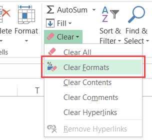
To do this, you need to use the ‘Clear Formats’ option, which can be found in the Home tab in the editing group. It becomes visible when you click on the ‘Clear’ drop down.
Note there are other options as well – such as clear contents, clear comments, and clear Hyperlinks. In case you want to clear everything – use the ‘Clear All’ option.
What is Conditional Formatting?
Conditional Formatting allows you to format a cell based on the value in it. For example, if you want to highlight all the cells where the value in less than 30 with a red color, you can do that with Conditional Formatting.
You can read more about Conditional Formatting here.
How would you highlight cells with negative values in it?
You can do this using conditional formatting.
Here are the steps:
- Select the cells in which you want to highlight the cells with negative value.
- Go to the Home tab and click on Conditional Formatting option.
- Go to Highlight Cell Rules and click on ‘Less Than’ option.
- In the ‘Less Than’ dialogue box, specify the value as 0 and the formatting.
How would you highlight cells with duplicate values in it?
You can do this easily using conditional formatting. Here are the steps:
- Select the data in which you want to highlight duplicate cells.
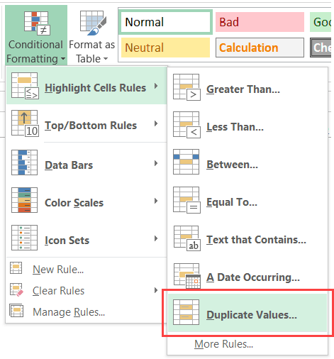
- Go to the Home tab and click on Conditional Formatting option.
- Go to Highlight Cell Rules and click on ‘Duplicate Values’ option.
How would you highlight cells with errors in it?
In Excel, there can be different types of errors – such as #N/A, #DIV/0!, #VALUE!, #REF!, #NAME, and #NUM.
You can highlight all the cells that contain any of these errors using conditional formatting.
Here are the steps to highlight cells with errors:
- Select the data in which you want to highlight the cells with errors.
- Go to the Home tab and click on Conditional Formatting option.
- Click on ‘New Rule’.
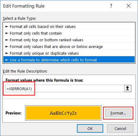
- In the New Formatting Rule dialog box, select ‘Use a formula to determine which cells to format’ option.
- In the formula field, enter =ISERROR(A1), where A1 is the active cell in the selection.
- Click on the Format button and specify the color in which you want to highlight the cells.
- Click OK.
How can you make text invisible in Excel?
There are multiple ways to do this:
- You can simply make the font white and it will appear as if it’s invisible.
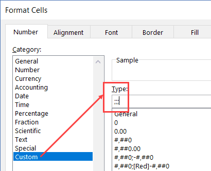
- [Better Way] You can change make the text invisible by changing the custom format. Here are the steps to do this. Select the cell, press Control + 1 (hold the control key and press 1). This will open the Format Cells dialog box. In the Custom option, type ;;; in custom option field. This will make the text invisible (but it will still be there).
Excel Formula Questions
Below are some common Excel formula questions for interviews (click on the question to view the answer to it).
What is the order of operations used when evaluating formulas in Excel?
Following is the order of precedence in Excel formulas:
- Parenthesis (Brackets)
- Exponentiation (^)
- Multiplication or Division – both have equal precedence and is evaluated based on whichever comes first
- Addition or Subtraction – both have equal precedence and is evaluated based on whichever comes first
An easy way to remember this is by the acronym PEMDAS – which is the first alphabet of each operator.
What is the difference between a function and a formula in Excel?
A formula is a user-defined expression that calculates a value. A function is pre-defined built-in operation that can take the specified number of arguments. A user can create formulas that can be complex and can have multiple functions in it.
For example, =A1+A2 is a formula and =SUM(A1:A10) is a function.
What, according to you, are the top 5 functions in Excel?
This question is often asked to understand comfort of a candidate with Excel functions.
While there are 450+ functions in Excel and there is no set criteria to select the top five, here are the ones I believe are worthy:
I have chosen the above functions as these are not very basic and are quite useful for someone who does analysis in Excel.
You can also consider the following functions – SUMPRODUCT, TEXT, SUM, AVERAGE, LEN/LEFT/RIGHT/MID.
Again, there is no right or wrong answer to this. Just make sure you know the functions that you mention.
You can find detailed explanations of most popular Excel functions here.
Also read: Excel Formulas Not Working
What is the difference between absolute and relative cell references?
In Excel reference refers to a cell reference – such as A1 or range reference – such as A1:A10.
Relative References: These are cell references that change when you copy and paste the formula that has the references. To give you a simple example, if you put =A10 in cell A1, and then you copy cell A1 and paste it in cell A2, the reference would change to A11. This happens as this is a relative cell reference and it changes relative to the cell it’s copied from.
Absolute References: These are the references that remain the same and don’t change copy and paste the formula that has the references. For example, if you put =$A$10 in cell A1 and then copy cell A1 and paste it in cell A2, the reference would still remain $A$10. The $ sign before the column alphabet and the row number makes it absolute.
You can read more about absolute and relative references here.
What are the different types of errors you can encounter in Excel?
When working with Excel, you can encounter the following six types of errors:
- #N/A Error: This is called the ‘Value Not Available’ error. You will see this when you use a lookup formula and it can’t find the value (hence Not Available).
- #DIV/0! Error: You’re likely to see this error when a number is divided by 0. This is called the division error.
- #VALUE! Error: The value error occurs when you use an incorrect data type in a formula.
- #REF! Error: This is called the reference error and you will see this when the reference in the formula is no longer valid. This could be the case when the formula refers to a cell reference and that cell reference does not exist (happens when you delete a row/column or worksheet that was referred in the formula).
- #NAME ERROR: This error is likely to a result of a misspelled function.
- #NUM ERROR: Number error can occur if you try and calculate a very large value in Excel. For example, =194^643 will return a number error.
How can you tackle errors when working with Excel Formulas?
There are various ways you can tackle the errors in Excel:
- You can highlight the errors using conditional formatting. This requires using the ISERROR function in conditional formatting.
- You can use the IFERROR function in Excel to get a specific value in case the formula returns an error.
- You can use ISERROR to get TRUE in case there is an error and FALSE in case there is not.
- You can use IFNA function to tackle the #N/A error.
Which function would you use to get the current date and time in Excel?
The following functions can be used:
- TODAY() – This function takes no argument and would return the current date value.
- NOW() – This function takes no argument and would return the current date and time value.
Remember that that dates and time are stored as numbers in Excel. So you can perform operations such as addition/subtraction with these dates.
How can you combine the text from multiple cells using a formula?
To combine text from different cells, you can use any one of the following three methods:
- TEXTJOIN function – If you’re using Office 365 subscription, you will have the TEXTJOIN function available in your version. Click here to read how it works.
- CONCATENATE function – If you want to combine values in cell A1 and A2, you can use the formula =CONCATENATE(A1,A2)
- Ampersand (&) operator: This works just like the CONCATENATE function. To combine text strings in cell A1 and A2, use the formula =A1&A2
You can read more about joining strings in Excel here.
What formula would you use to find the length of a text string in a cell?
You can find the length of a string in a cell using the LEN function.
For example, if you want to know the length of the string in cell A1, you can use the formula =LEN(A1)
What is the syntax of the VLOOKUP function?
VLOOKUP is definitely one of the most popular Excel functions. And this is also one of the most asked Excel question that I have seen in interviews.
Here is the VLOOKUP syntax:
=VLOOKUP(lookup_value, table_array, col_index_num, [range_lookup])
- lookup_value – this is the look-up value you are trying to find in the left-most column of a table. It could be a value, a cell reference, or a text string. In the score sheet example, this would be your name.
- table_array – this is the table array in which you are looking for the value. This could be a reference to a range of cells or a named range. In the score sheet example, this would be the entire table that contains score for everyone for every subject
- col_index – this is the column index number from which you want to fetch the matching value. In the score sheet example, if you want the scores for Math (which is the first column in a table that contains the scores), you’d look in column 1. If you want the scores for Physics, you’d look in column 2.
- [range_lookup] – here you specify whether you want an exact match or an approximate match. If omitted, it defaults to TRUE – approximate match.
If you’ve time, I recommend going this VLOOKUP function guide I created with 10 practical examples.
How would you get rid of leading / trailing / double spaces in a text in Excel?
To get rid of leading, trailing, and double spaces, you need to use the TRIM function.
For example, if you have a text string in cell A1 and you want to remove the spaces, you can use the following formula:
=TRIM(A1)
Note that it doesn’t remove single spaces between words.
Excel TRIM function does a good job in removing spaces in Excel, however, it fails when you have non-printing characters (such as line breaks) in your data set. To remove non-printing characters, you can use a combination of TRIM and CLEAN functions.
If you have some text in cell A1 from which you want to remove spaces, use the below formula:
=TRIM(CLEAN(A1))
You can read more about it here.
What are the known limitations of the VLOOKUP function?
The VLOOKUP function is mighty useful, but it also has a few limitations:
- It can not be used when the lookup value is on the right. For VLOOKUP to work, the lookup value should always be in the left-most column. Now this limitation can be overcome by using it with other formulas, it tends to make formulas complex.
- VLOOKUP would give a wrong result if you add/delete a new column in your data (as the column number value now refers to the wrong column). You can make the column number dynamic, but if you planning to combine two or more functions, why not use INDEX/MATCH in the first place.
- When used on large data sets, it can make your workbook slow.
You can read my comparison of VLOOKUP Vs. INDEX/MATCH here.
Here are some examples of using the INDEX MATCH combo in Excel.
When would you use the SUBTOTAL function?
When you’re working with tabular data, you can use the SUBTOTAL function to get variety of subtotals – such as AVERAGE, COUNT, MAX, MIN, STDEV.
One of the highlights of SUBTOTAL function is that it allows you to ignore hidden/filtered cells. So if you have a huge data set and you filter it based on a criteria or hide some rows, SUBTOTAL function will automatically update to give you the result from the visible cells only.
Of course, if you don’t want the data of filtered/hidden cells to be ignored, you can do that too.
Also read: Excel Weighted Average Formula
What are volatile functions? Can you name a few?
A volatile function recalculates the formula again and again (whenever there is any change in the worksheet). This can slow down the workbook considerably.
A very simple example of a volatile function is the NOW() function (to get the current date and time in a cell). Whenever you edit any cell in a worksheet, it gets recalculate. This is fine if you have a small data set and less number of formulas, but when you have large spreadsheets, this could significantly slow down the processing.
Here is a list of volatile formulas:
- Highly volatile: RAND(), NOW(), TODAY()
- Almost volatile: OFFSET(), CELL(), INDIRECT(), INFO()
BONUS TIP: Conditional formatting is also volatile. You should use it only the cells where it’s needed.
Excel Keyboard Shortcuts
Below are some common Excel interview questions about keyboard shortcuts that you might get asked in an interview (click on the question to view the answer).
What are the most useful keyboard shortcuts you use?
There are hundreds of Excel keyboard shortcuts. I am listing my top five shortcuts, but in case you have your own, feel free to use that.
- CONTROL D to fill down the content from the cell above.
- SHIFT Spacebar to select entire row (or CONTROL + Spacebar to select entire column).
- CONTROL – to delete cells/row/column. This opens the delete dialog box where you can choose what to delete.
- CONTROL ; to insert current date (CONTROL SHIFT ; inserts the current time).
- CONTROL PAGEUP/PAGEDOWN to cycle through the worksheets.
You can read the following tutorials in case you want to more keyboard shortcuts:
What is the shortcut for opening the find and replace dialog box
- CONTROL F – This opens the Find and Replace dialog box with the Find tab selected.
- CONTROL H – This opens the Find and Replace dialog box with the Replace tab selected.
What is the shortcut for spell check?
F7 – This opens the spell-check dialog box.
What is the shortcut to quickly auto-sum rows/columns?
ALT =
If you have numbers in a column/row, you can quickly get the sum by using this Excel keyboard shortcut.
What is the shortcut to open a new Excel workbook?
CONTROL N
This works only when you have the Excel application open.
How can you select all the cells in the worksheet
You can use CONTROL A A – hold the control key and hit the A key twice.
In case you don’t have any data around the active cell, hitting the A key once would select the entire worksheet. But in case there is data, hitting the A key once select the entire data and hitting it again then selects all the cells in the worksheet.
How would you insert a new line in the same cell?
To insert a new line in the same cell, use the shortcut ALT Enter – hold the ALT key and press enter.
What’s the shortcut to insert a comment in Excel?
SHIFT F2
Select the cell in which you want to add the comment, hold the ALT key press the F2 key.
In case you have selected a range of cells, it will insert the comment in the active cell only.
Excel Pivot Table Questions
Below are some common Excel interview questions about Pivot Table that you might get asked in an interview (click on the question to view the answer).
What is a Pivot Table, and when would you use one?
A Pivot Table is a feature in Microsoft Excel that allows you to quickly summarize huge data sets (with a few clicks).
Even if you’re absolutely new to the world of Excel, you can easily use a Pivot Table. It’s as easy as dragging and dropping rows/columns headers to create reports.
To give you an example, if you have the 10,000 rows sales data from four different regions, you can use a Pivot Table to instantly find what are the total sales in each region. If you want to further drill down and see what are the sales of each product in each region, you can easily do that (it’s literally as easy as dragging a data point in a box).
You can read more about Pivot Tables here.
What are the various sections in a Pivot Table?
A Pivot table is made up of four different sections:
- Values Area: This is the area where the values are reported.
- Rows Area: The headings to the left of the Values area makes the Rows area.
- Columns Area: The headings at the top of the Values area makes the Columns area.
- Filter Area: It is an optional filter that you can use to further drill down in the data set.
What are slicers?
Slicers were introduced in Pivot Table in the 2010 version of Excel.
A Pivot Table Slicer enables you to filter the data when you select one or more than one options in the Slicer box (as shown below).
What is a Pivot Chart
When you create a Pivot Table, you get the summary of your data. You can also plot this summary in a chart that is connected to the data.
This chart is called the Pivot Chart.
One big benefit of using a Pivot Chart is that it updates when you change the Pivot Table layout. For example, if you have the total sales by region, and you update the Pivot Table to show sales data for each product in the regions, the Pivot Chart would accordingly update.
What are the difference between Pivot Charts Vs Regular Charts?
While Pivot Charts are amazing and come with the ability to update when the Pivot Table updates, these are not as flexible as the regular charts.
In general, you can do a lot of customization in a regular Excel chart, but not in a Pivot chart. Also, if you customize a Pivot Chart, and then update the Pivot Table, you are likely to lose the customization.
Despite the limitations, Pivot Charts are useful and can help create quick views from a Pivot Table.
How can you refresh a Pivot Table?
To refresh a Pivot table, click on any cell in the Pivot Table, right-click and select Refresh.
Another way of refreshing a Pivot Table is to select any cell in the Pivot Table. It will enable the Pivot Table Tools tab. In the Analyze tab, click on ‘Refresh’.
You can read more about refreshing the Pivot Table here.
Can you group dates in Pivot Tables?
If you have date wise records, you can easily group these into the following segments:
- Years
- Quarters
- Months
- Weeks
- Days
- Hours / Minutes / Seconds
The option to group data in Pivot Table is in the Analyze tab, which becomes visible when you select a cell in the Pivot Table in the Rows area.
You can read more about grouping dates in Pivot Table here.
What is a Pivot Cache?
Pivot Cache is something that automatically gets generated when you create a Pivot Table.It is an object that holds a replica of the data source. While you can’t see it, it is a part of the workbook and is connected to the Pivot Table. When you make any changes in the Pivot Table, it does not use the data source, rather it uses the Pivot Cache.The reason a pivot cache gets generated is to optimize the pivot table functioning. Even when you have thousands of rows of data, a pivot table is super fast in summarizing it. You can drag and drop items in the rows/columns/values/filters boxes and it will instantly update the results.Pivot Cache enables this fast functioning of a pivot table.
Can you make a Pivot Table from multiple tables?
Yes, you can create one Pivot Table from multiple different tables. However, there needs to be a connection in these tables.
For example, if you have two tables, one that has date, Product ID and sale value, and another which has Product ID and Product Name, then you can combine these as the common column in Product ID.
Once you have connected these tables, you can create a Pivot table from these.
A crucial part of this is to set-up table relationships (where you specify the relationship between 2 tables).
You can read more about this here.
What are Calculated Fields in Pivot Table?
A calculated field allows you to add a column to the Pivot Table data where you can use the existing columns to do some calculations.
Let me give you a simple example.
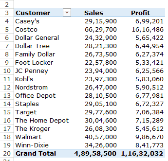
Suppose you have a data set of retailers and you’ve created a Pivot Table as shown below:
The above Pivot Table summarizes the sales and profit values for the retailers.
Now, what if you also want to know what was the profit margin of these retailers (where the profit margin is ‘Profit’ divided by ‘Sales’).
You have a couple of options:
- You can go back to the original data set and add this new column. This is feasible but not the best solution as it alters the original data set and increases file size.
- You can do this calculation outside of the Pivot Table. This is alright if your Pivot Table is static, but if you update the table or change the layout, you’ll need to do the calculations again.
- You add a calculated field.
Consider Calculated Field as a virtual column that you have added using the existing columns from the Pivot Table.
There are a lot of benefits of using a Pivot Table Calculated Field:
- It doesn’t require you to handle formulas or update source data.
- It’s scalable as it will automatically account for any new data that you may add to your Pivot Table. Once you add a Calculate Field, you can use it like any other field in your Pivot Table.
- It easy to update and manage. For example, if the metrics change or you need to change the calculation, you can easily do that from the Pivot Table itself.
You can read more about the Pivot Table Calculated Field here.
Excel Charting Questions
Below are some common Excel interview questions about charting that you might get asked in an interview (click on the question to view the answer).
What is a Column chart?
A column chart is made up of vertical bars that is used to compare values over time or two compare values in different categories.
For example, you can use it to see how the sales have done over the years. Or you can use it to compare which product category has done better sales. Since you can see all the vertical bars at one go, it is easier to visually see and compare.
You can also create clustered column charts, where you can have multiple columns for the same category or year (something as shown below).
What is a Bar chart?
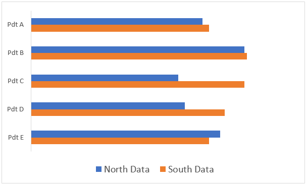
A bar chart is made up of horizontal bars that is used to compare values in different categories.
For example, you can use it to compare which product category has done better sales. Or what has been the response of a survey.
You can also create clustered bar charts, where you can have multiple bars for the same category (something as shown below).
What is a Line chart?
Line chart are useful when you want to show a trend over the years (or other time periods such as weeks, months, or quarters).
You can have multiple lines in a line chart. This would allow you to compare different categories over the same period of time (something as shown below).
What is a Scatter chart?
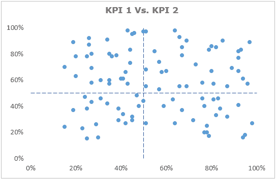
A scatter chart is used to compare two sets of values. For example, you can have data of different products on two KPIs, and you can plot the data on a scatter chart (as shown below).
This allows you to see what products are doing well on both the KPIs (the top right quadrant) or doing bad on both the KPIs (bottom-left quadrant).
You can see an example of scatter chart in action in the KPI Dashboard here.
Are Pie charts good? Should it used in reports/dashboard?
There are two school of thoughts.
There are some who completely hate Pie chart and recommend never to use these (such as this article). And then there are some (including myself), who sometime use Pie charts in dashboards in reports.
There are many managers who are comfortable with pie charts and find these easy to read. So if you want to show a breakup of revenue by division (where you have only a few divisions), then you can use a pie-chart.
Let me be clear. Pie chart can be completely replaced by a bar chart. There is no additional benefit of using it. But in some cases, Pie charts make a good story (for example showing that one division is bringing in ~75% of the revenue as shown below).
You should avoid using Pie charts:
- In case the difference in values in not significant. The difference is better visualized by a bar chart.
- In case there are too many parts in a pie chart. In such cases, it can look cluttered.
What is a Waterfall chart? When would you use it?
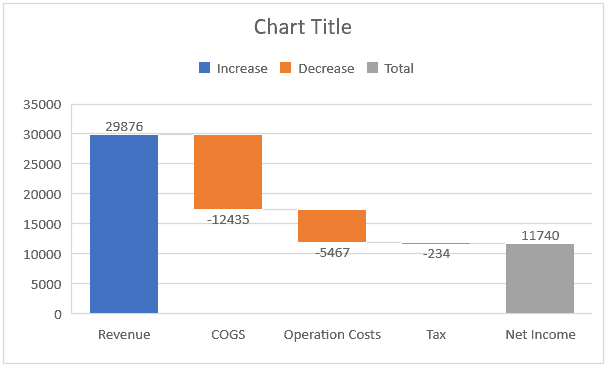
A waterfall chart shows different values (positive and negative) that lead to the final result value. For example, if you’re analyzing companies net income, you can have all the cost components shown in the waterfall chart.
This will help you visually see how the value from revenue to net income is obtained when all the costs are deducted.
What are Combination charts?
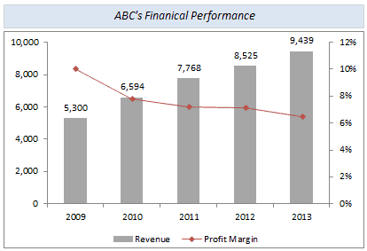
Combination charts are those where you combine more than one chart type. A popular example of this is showing bar chart with a line chart.
Combination charts let you present and compare two different data-sets that are related to each other. For example, you may be interested in plotting the revenue figures of a company, and at the same time, also be able to show how the profit margin has changed. A combination chart (as shown below) is an apt way of doing this.
What is a secondary axes in a chart?
In a chart, there is a Y axis where you show the scale on which you can measure the chart (be a bar chart or line chart or others).
In cases where you have two show two different types of data set with a significant difference in value, you can use the secondary axes.
To give you an example, if you want to show the revenue and net income margin in the same chart, you need to show two different axes. This is because revenue numbers can be in thousands or millions, but net income margin would be in percentage and always less than 100%. In this case, you need to have two axes, one that shows scale for revenue and one that scale for net income margin.
So when you add another axes, it is called the secondary axes. In the below figure, the axes on the right is the secondary axes.
What is a Bullet chart? When should we use it?
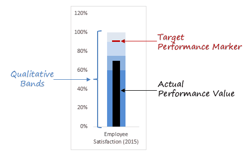
Bullet charts were designed by the dashboard expert Stephen Few, and since then it has been widely accepted as one of the best charting representations where you need to show performance against a target.
One of the best things about bullet charts is that it is power-packed with information and takes little space in your report or dashboards.
Below is an example of a bullet chart:
Note that bullet charts are not a default chart type in Excel, and you need to use a number of steps to create these.
You can read more about bullet charts here.
Excel Data Analysis Questions
Below are some common Excel interview questions about Data Analysis that you might get asked in an interview (click on the question to view the answer).
How to replace one value with another in Excel?
You can replace one value with another using the FIND & REPLACE feature in Excel.
To do this, select the data set and use the keyboard shortcut – CONTROL H (hold the control key and then press H). This will open the Find & Replace dialog box.
In this dialog box, you can specify the value you want to change and the replacement value.
If you’re interested in learning more about Find and Replace, click here.
What kind of data filters are available in Excel?
In Excel, you can filter a data set based on the kind of data.
The following types of data filters are available in Excel:
- Text Filter
- Number Filter
- Date Filter
You can apply filter to a data set, by selecting the data, then clicking the Home tab and clicking on the Filter icon.
When you have tabular data and you apply filters, based on the data in the column, Excel shows you the relevant filter. For example, if you have text data, it will show you filters related to text (such as text contains, begins with, ends with, etc.).
You c
How can you sort data in Excel?
There is a sorting feature in Excel that can sort data based on text, numbers, or colors.
Here are some ways to sort data in Excel:
- Select the data and click on one of the two sort icons in the Data tab.
- Select the data and click on the Sort icon. It will open the sort dialog box and you can specify the column to sort and the criteria (ascending/descending).
- Apply data filter, and click on the filter. Along with the filter options, it also shows the data sorting options.
You can read more about data sorting here.
What is data validation?
Data Validation allows you to enter only that data in a cell that satisfies a criteria.
For example, if you want to only have numbers entered in a cell, then you can use Data validation to do this. In case any one enters something other than numbers, Excel will show an error and not allow that.
Data validation options are available in the data tab.
You can read more about data validation here.
Data validation can be really helpful when you’re creating forms in Excel. For example, if you want a user to enter only their age, you can use Data Validation to make sure the cell accepts a numeric value only.
How can you transpose a data set in Excel?
There are two popular ways to transposing data in Excel:
- Using Paste Special dialog box.
- Using the Transpose Function.
With Paste Special dialog box, you need to first copy the data that you want to transpose, select the cell where you want to paste it, right-click and go to Paste special, and select the Transpose option (as shown below).
You can read more about transposing data in Excel here.
How can you select all blank cells in Excel?
If you work with a data set that has blank cells in it, you can easily select these cells in Excel. Once selected, you can choose to highlight these, delete these, or add some value to it (such as 0 or NA).
To do this, you need to use the Go To Special dialog box in Excel.
Here are the steps to select all blank cells in Excel:
- Select the entire data set (including blank cells)
- Press F5 (this opens the Go To dialog box)
- Click the ‘Special’ button (this opens the Go To special dialogue box)
- Select Blanks and click OK (this selects all the blank cells in your data set)
You can read more about selecting blank cells in Excel here.
How can you remove duplicates from a data set?
Excel has an in-built functionality that allows you to remove duplicate cells/rows in Excel.
You can find the option to remove duplicates in the Data tab.
Here are the steps to remove duplicates in Excel:
- Select the data.
- Click the Data tab and then click on the Remove Duplicates option.
- In the Remove Duplicates dialog box, if your data has headers, make sure the ‘My data has headers’ option is checked. Select the column from which you want to remove duplicates.
- Click OK
You can read more about removing duplicates in Excel here.
What is an advanced Filter in Excel?
Excel Advanced Filter – as the name suggests – is the advanced version of the regular filter. You can use this when you need to use more complex criteria to filter your data set.
Here are some differences between the regular filter and Advanced filter:
- While the regular data filter will filter the existing data set, you can use Excel advanced filter to extract the data set to some other location as well.
- Excel Advanced Filter allows you to use complex criteria. For example, if you have sales data, you can filter data on a criterion where the sales rep is Bob and the region is either North or South.
You can read more about Excel Advanced Filter here.
Can you sort multiple columns at one time?
Yes, you can sort multiple columns in Excel.
With multiple sorting, the idea is to sort a column and then sort the other column while keeping the first column intact.
Below is an example of multiple level sorting in Excel.
Note that Column A is sorted first in this case and then Column B is sorted. The final result has Column A values sorted, and Column B sorted for each item in Column A.
To do multiple level sorting, you need to use the Sort dialog box. To get that, select the data that you want to sort, click the Data tab and then click on the Sort icon.
In the Sort dialog box, you can specify the sorting details for one column, and then to sort another column, click on ‘Add Level’ button. This will allow you to sort based on multiple columns.
You can read more about multiple-column data sorting here.
What is a one-variable data table?
One variable Data Table in Excel is most suited in situations when you want to see how the final result changes when you change one of the input variables.
For example, if you want to know how much on monthly installment change if you increase/decrease the number of months, you can set up a one-variable data table for it. This can be useful when you want to keep the monthly payment less than $500 and know what all options you have (6 months, 9 months, 12 months, etc.)
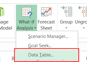
The option to set One-Variable data table is in the Data tab, in the What-if Analysis drop down.
You can read more about One-variable data table here.
What is a two-variable data table?
Two variable Data Table in Excel is most suited in situations when you want to see how the final result changes when you change two of the input variables.
For example, if you want to know how much on monthly installment change if you increase/decrease the number of months and the interest rate.
You can set up a two-variable data table for it that will show you a the final monthly installment based on different combinations of interest rate and number of months. This can be useful when you want to keep the monthly payment less than $500 and know what all options you have.
The option to set Two-Variable data table is in the Data tab, in the What-if Analysis drop down.
You can read more about Two-variable data table here.
What is Scenario Manager?
Scenario Manager in Excel can be the tool of choice when you have multiple variables, and you want to see the effect on the final result when these variables change.If you only have one or two variables changing, you can create a one variable or two-variable data table. But if you have 3 or more than 3 variable that can change, then scenario manager is the way to go.
For example, if you’re a regional sales manager and have four areas under you, you can use scenario manager to create different scenarios (such as):
- None of the area shows any growth in sales.
- Area A grows 10% but the other 3 don’t grow.
- Area A and B grow by 10%, but other two don’t grow.
You get the idea.. right?
With scenario manager in Excel, you can easily create the scenarios and analyze these one by one or as a summary of all the scenarios.
You can read more about scenario manager here.
What is Goal Seek?
Goal Seek in Excel, as the name suggests, helps you in achieving a value (the goal) by altering a dependent value.
For example, if you’re buying a car and you want to know how many month’s installment you should opt-for so that your monthly payment is not more than $500, you can do this using Goal seek.
You can read more about Goal Seek here.
What is a Solver?
Solver in Excel is an add-in that allows you to get an optimum solution when there are many variables and constraints. You can consider it to be an advanced version of Goal Seek.
With Solver, you can specify what the constraints are and the objective that you need to achieve. It does the calculation in the back-end to give you a possible solution.
You can read more about Solver here.
Excel VBA Questions
Below are some common Excel interview questions about VBA that you might get asked in an interview (click on the question to view the answer).
What is VBA?
VBA stands for Visual Basic for Applications. It’s the programming language that you can use to automate tasks in Excel.
What are the benefits of using VBA in Excel?
While Excel has a lot of amazing features and functionalities, it may not have everything you need.
VBA allows you to enhance Excel’s ability by creating codes that can automate tasks in Excel. Below are some of the things you can do this VBA:
- Automate a set of tasks and save time.
- Create your own Excel functions (in case existing functions are not enough).
- Create and share your codes with other people so they can also automate tasks and save time.
- Create custom applications.
What is a macro in Excel?
A macro is a set of instructions written in the VBA language that Excel can understand and execute. A macro can be as simple as a single line or can be thousands of line long.
In many cases, people tend to use VBA code and macro interchangeably.
How can you record a macro in Excel?
Even if you know nothing about VBA, you can still create some macros and automate your work.
You can do this by recording a macro.
When you record a macro, Excel closely watches the steps you’re taking and notes it down in a language that it understands – which is VBA.
Now, when you stop the recording, save the macro, and run it, Excel simply goes back to the VBA code it generated and follows the exact same steps.
This means that even if you know nothing about VBA, you can automate some tasks just by letting Excel record your steps once and then reuse these later.
You can record a macro by using the Record Macro option which is available in the Developer tab in the ribbon.
Once you record the macro, Excel stores it with the name you specify and then you can easily reuse it as many times as you want.
You can read more about recording a macro here.
What are limitations of recording a macro in Excel?
While recording a macro is a great way to quickly generate code, it has the following limitations:
- You can’t execute a code without selecting the object. If you want the macro recorder to go to the next worksheet and highlight all the filled cells in column A, without leaving the current worksheet, then it won’t be able to do this. It’s because if I ask you to do this, even you won’t be able to do that (without leaving the current sheet). And if you can’t do it yourself, how will the macro recorder capture your actions. In such cases, you need to manually go and create/edit the code.
- You can’t create a custom function with a macro recorder. With VBA, you can create custom functions that you can use in the worksheet as regular functions. You can create this by writing the code manually.
- You can’t run codes based on Events. In VBA you can use many events – such as opening a workbook, adding a worksheet, double-clicking on a cell, etc, to run a code associated with that event. You can’t use a macro recorder to do this.
- You can’t create loops with a macro recorder. When you manually enter the code, you can leverage the power of loops in VBA (such as For Next, For Each Next, Do While, Do until). But you can’t do this when you record a macro.
- You can’t analyze conditions: You can check for conditions within the code using macro recorder. If you write a VBA code manually, you can use the IF Then Else statements to analyze a condition and run a code if true (or another code if false).
What is a UDF in Excel VBA?
A UDF is a User Defined Function in VBA. These are also called custom functions.
With VBA, you can create a custom Function (UDF) that can be used in the worksheets just like regular functions.
These are helpful when the existing Excel functions are not enough. In such cases, you can create your own custom UDFs to cater to your specific needs.
You can read more about User Defined Functions here.
What are Events in VBA?
In Excel VBA, an event is an action that can trigger execution of the specified macro.
For example, when you open a new workbook, it’s an event. When you insert a new worksheet, it’s an event. When you double-click on a cell, it’s an event.
There are many such events in VBA, and you can create codes for these events. This means that as soon as an event occurs, and if you have specified a code for that event, that code would instantly be executed.
Excel automatically does this as soon as it notices that an event has taken place. So you only need to write the code and place it in the correct event subroutine.
You can read more about the Excel VBA Events here.
What are some of the useful loops in VBA?
There are the following loops in Excel VBA:
- For Next Loop
- Do While Loop
- Do Until Loop
- For Each Next Loop
You can read more about Excel VBA Loops here.
What are the different ways to run a macro in Excel?
You can use the following ways to run a macro in Excel:
- Assign the Macro to a Shape
- Assign the Macro to a Button
- Run a Macro from the Ribbon (Developer Tab)
- Run a Macro from the VB Editor
- Run a Macro using a Keyboard Shortcut
- Call a Macro from another Macro
You can read more about running a macro here.
What are UserForms?
A UserForm is a dialog box that you can design and build in Excel VBA.
Once created, these can be used in many ways in the Excel worksheet area:
- You can use it to get input from the user.
- You can make a form and record the entries in Excel.
- You can add buttons to the UserForm and give options to the user. You can also code these buttons so every time a user clicks on a button, a specific macro is executed.
What are add-ins?
An add-in is a file that you can load with Excel when it start.
When you create an add-in and install it in Excel, it opens whenever the Excel application opens. You can have many different macros in an add-in and whenever you open Excel, these codes are available for use.
This is useful as you can create an add-in and becomes available to all the workbooks. So if there are some tasks that you need to do often, you can automate these by writing a macro and then saving these as add-ins. Now no matter what Excel you open, you can use the macro.
Another benefit of add-in is that you can share the add-in file with others as well. All they need to do is install it once and they will also have the same macros available to them
You can read more about creating an add-in here.
Excel Dashboard Questions
Below are some common Excel interview questions about dashboards that you might get asked in an interview (click on the question to view the answer).
What is difference between a dashboard and a report?
A report is meant to provide relevant data. It could be a report that has all the data or can also have a few charts/visualizations. Examples of reports can be sales transaction data or employee survey data.
A dashboard is meant to answer questions using the data. It could be to show which regions are performing better in sales or which areas are lagging in terms of employee feedback. These dashboards could be static or interactive (where the user can make selections and change views and the data would dynamically update).
You can read more about Excel Dashboards here.
What are some of the questions you should ask a client/stakeholder before creating a dashboard?
While the questions would depend on a case to case basis, there are few high-level questions that you should ask when creating a dashboard in Excel.
- What is the Purpose of the Dashboard?
- What are the data sources?
- Who will use this Excel Dashboard?
- How frequently does the Excel Dashboard needs to be updated?
- What version of Office does the client/stakeholder uses?
There can be many such questions. The intent here is to be clear on what the dashboard needs to be and what purpose it serves.
What are some interactive controls you can use in dashboards?
Excel has a number of interactive tools that can be used in a dashboard:
Apart from these regular interactive tools, you can also use VBA to add more functionality to your dashboard.
What are some useful chart types that you can use in a dashboard?
One of the need when creating a dashboard is to show relevant data with visuals. Charts that can tell a good story and show relevant information are more suited for dashboard.
Since a dashboard is usually expected to fit in a single screen, there is limited space for data and visuals. In such cases, combinations charts come handy.
The following charts can be useful when creating a dashboard:
- Combination charts
- Scatter Charts
- Bullet Chart
- Waterfall chart
- Heat Maps
What are some best practices when creating a dashboard in Excel?
Here are some best practices when creating dashboard in Excel:
- Convert Tabular Data into Excel Tables: Creating dashboards using an Excel Table as the data source is way easier. Unless you have extremely strong reasons against it, always convert back-end data into an Excel Table.
- Numbering your Charts/Section: This helps when you’re presenting the dashboard and referring to different charts/tables. It’s easier to ask people to focus on chart numbered 2, instead of saying the line chart or bar chart on the top-left.
- Restrict Movement in the dashboard area: While an Excel worksheet is huge, it’s better to remove all the rows/columns except the ones that have your dashboard.
- Freeze Important rows/column: In case you want some rows/columns to always be visible, you can freeze these.
- Make Shapes/Charts Stick: A user may end up changing row/column width. You don’t want the shapes and charts to get misaligned and move from their original place. So it’s better to make them stick to their position.
- Provide a User Guide: It’s a good idea to include a separate sheet that has the details on how to use the dashboard. This becomes more useful when you have interactive controls in the dashboard.
- Save Space with Combination Charts: Since there is limited space in a dashboard (as you need to fit it in one screen), using combination charts can save you space.
- Use Symbols & Conditional Formatting: You can make dashboard more visual and easy to read by using symbols and conditional formatting. For example, it’s easier to see the lowest value in a table when it’s highlighted in red, instead of going through all the values one by one.
- Use colors wisely to show contrast: When you want to highlight a data point in a table or a bar in the chart, it better to make it stand out by highlighting it in eye-catching color.
Other Excel Questions
These are the questions that I could not fit in any of the above categories. So I am putting all these together here (click on the question to view the answer).
What is an Excel Table?
An Excel Table is a feature in Excel. This is not the same as tabular data.
When you convert tabular data into an Excel Table, there are a few additional features that get added to it that can be really useful.
According to Microsoft Help Site – “A table typically contains related data in a series of worksheet rows and columns that have been formatted as a table. By using the table features, you can then manage the data in the table rows and columns independently from the data in other rows and columns on the worksheet.”
You can read more about Excel Tables here.
What are the benefits of using Excel Table?
When you convert tabular data into Excel Table, the following features are automatically added to the data:
- You can use the filter icon on each column header to sorting and filter the data.
- You can easily apply styles to a table and format it. There are a lot of in-built styles available that you can use with a single click.
- You can use Table Name and Column Names instead of cell references in formulas.
- When you add a new row/column to the tabular data, the Excel Table automatically expands to cover the new row/column as a part of it. And since you can use Table/Column names in formulas, you don’t need to go and update formulas when new rows/columns are added. Excel Table automatically accounts for it.
What are structured references?
When you use an Excel Table, you don’t need to use the cell references. Instead, you can use the Table name or the column names. These references are called structured references.
What are the commonly used file formats in which an Excel file can be saved?
There are a lot of file formats in which you can save your Excel workbook. Some commonly used ones are:
- .XLS
- .XLSX
- .XLSM (when you file has macros)
- .CSV
- .XLB (binary format)
- .XLA (for add-ins)
How to reduce the size of an Excel file?
There are many ways you can reduce the file size of an Excel Workbook:
- Delete unused data
- Delete unused worksheets
- Remove images or compress these images
- Remove unnecessary formatting
- Remove Pivot Tables you don’t need. This will also help clear the Pivot Cache.
- Save file in the .XLSB format
Read more: 8 ways to reduce file size in Excel
What steps can you take to handle slow Excel workbooks?
You can use the following techniques to handle slow Excel workbooks:
- Avoid Volatile Functions such as INDIRECT, OFFSET, etc.
- Use Helper Columns instead of array formula
- Use Conditional formatting only when absolutely necessary (as it is volatile too).
- Use Excel Tables and Named Ranges.
- Convert Unused Formulas to Values.
- Keep All Referenced Data in One Sheet.
- Avoid Using Entire Row/Column in References.
- Use Manual Calculation Mode.
You can read more how to handle slow Excel workbook here.
How many rows and columns are there in an Excel worksheet?
An Excel sheet (2007 and later versions) has:
- 16,384 columns
- 1,048,576 rows
How to add/delete rows in Excel?
To add new rows, right-click on any cell where you want insert the row and click on the Insert option. This will open a dialog box which you can use to insert new rows.
Similarly, to delete cells/rows/columns, select these, right-click and select Delete.
How can you zoom in or zoom out in Excel?
There are Zoom In and Zoom Out buttons in the status bar in Excel. You can click the plus sign to Zoom In and minus sign to Zoom Out.
You can also hold the Control Key and then use the scroll wheel in the mouse to Zoom in and Zoom out.
Also, in the View tab, there are option to Zoom in and out in Excel.
How to protect a sheet In Excel?
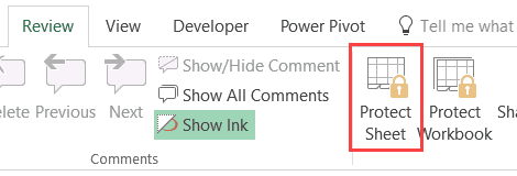
You can protect a sheet by clicking the Review tab and then clicking the Protect Sheet option.
This opens a dialog box where you can set a password. If you don’t want to set a password, you can leave it blank.
What are named ranges? What are its benefits?
A named range is a feature in Excel that allows you to give a cell or a range of cells a name. Now you can use this name instead of using the cell references.
Using a named range makes it easier when you’re working with formulas. This becomes specially useful when you have to create formulas that use data from multiple sheets. In such cases, you can create named ranges and then use these instead of the cell references.
You can give descriptive names to these named ranges – which also makes it easier to read and understand the formula. For example, you can use =SUM(SALES) instead of =SUM(C2:C11), which will instantly tell you what the formula is about.
You can read more about Named Ranges here.
Can you make the header rows/columns stick and be visible when you scroll?
When you’re working with large data sets, when you scroll to the bottom or to the right, the header rows and columns disappear. This sometimes makes it difficult to understand what a data point is about.
By using Freeze Panes option in Excel, you can make the header rows/columns be visible when you scroll away to the far off data points.
The Freeze Panes options are available in the View tab in the Excel ribbon.
You can read more about Excel Freeze Panes here.
How would you identify cells that have comments in it?
The cells that have a comments added to it are flagged by a small red triangle at the top-right of the cell. When you hover the cursor over the cell, the comments becomes visible.
How would you save an Excel worksheet as a PDF?
To save a worksheet as a PDF document, you can specify the file type as PDF when saving the file.
To do this, click on the File tab and then click on Save As.
In the Save As dialog box, select the location where you want to save the file and use the Save As type drop-down to select PDF. This will save the entire worksheet as a PDF document.
How to create a hyperlink in Excel?
To create a hyperlink, select the cell in which you want the hyperlink and use the keyboard shortcut Control K (hold the control key and press the K key).
This will open the Insert Hyperlink dialog box where you could specify the URL.
You can also get the option to add the hyperlink when you right-click on the cell.
When would you consider switching from automatic to manual calculation in Excel?
While in most cases automatic calculation mode is the way to go, in case you have a formula heavy file where recalculation takes a lot of time every time you change anything in the sheet, then you can switch to manual calculation.
Once you have switched to manual calculation, you need to refresh every time you want the sheet to recalculate.
What is Flash Fill?
Flash Fill is an amazing tool that was added in Excel 2013 and is available in all version after that.
You can use Flash Fill in Excel to make data entry easy. It’s a smart tool that tries to identify patterns based on your data entry and does that for you.
Some simple examples of using Flash Fill could be to get the first name from the full name, get name initials, format phone numbers, etc.
You can read more about Flash Fill here.
What is a Fill Handle?
Fill handle is a tool that you can use to autocomplete lists in Excel. For example, if you have to enter numbers 1 to 20 in cell A1:A20, instead of manually entering each number, you can simply enter the first two numbers and use the fill handle to do the rest.
Fill Handle is the small square you would see when you select two or more than two cells in Excel.
When you hover your cursor on Fill handle, the cursor changes to a plus icon. Now you can hold the left-mouse key and drag it to add more numbers in the series.
What are wildcard characters in Excel?
There are three wildcard characters in Excel:
- * (asterisk) – It represents any number of characters. For example, Ex* could mean Excel, Excels, Example, Expert, etc.
- ? (question mark) – It represents one single character. For example, Gl?ss could be Glass or Gloss.
- ~ (tilde) – It is used to identify a wildcard character (~, *, ?) in the text. For example, let’s say you want to find the exact phrase Excel* in a list. If you use Excel* as the search string, it would give you any word that has Excel at the beginning followed by any number of characters (such as Excel, Excels, Excellent). To specifically look for excel*, we need to use ~. So our search string would be excel~*. Here, the presence of ~ ensures that excel reads the following character as is, and not as a wildcard.
Wildcard characters are useful when you want to use it in formulas or while filtering data.
You can read more about Wildcard Characters here.
What is a Print Area and how can you set it in Excel?
A print area is a range of cells (contiguous or non-contiguous) that you designate to print whenever you print that worksheet. For example, instead of printing the entire worksheet, if I only want to print the first 10 rows, I can set the first 10 rows as the print area.
To set the Print Area in Excel:
- Select the cells for which you want to set the Print Area.
- Click on Page Layout tab.
- Click on Print Area.
- Click on Set Print Area.
You can read more about Print Area here.
How can you insert Page Numbers in Excel?
You can insert page numbers using the Page Setup dilaog box.
Here are the steps to do this:
- Click the Page Layout tab,
- In the Page Setup category, click on the dialog box launcher icon (which is the small tilted arrow icon at the bottom right of the group).
- In the Page Setup dialog box, click on Header/Footer tab.
- Select the Page Number format from the Footer drop-down.
You can read more about Page Numbers in Excel here.
While I have tried to keep this ‘Excel Interview Questions & Answer’ guide error-free, in case you find any errors in any of the questions, please let me know in the comments area.
Related: Free Online Excel Training (7-part video course)
You May Also Like the Following Excel Tutorials:




















It is definitely one of the best learning gifts of the new year. Thanks a ton, Sumit!
how to specify to select or exclude blank date in criteria range of advanced filter? =, ,, with date works.
Very useful
Really helpful
Want to learn sum.product as a vlook up …
Absolutely awesome. Thank you for sharing
Very helpful
Awesome information.
EXCELLENT KNOWLEDGE SOURCE
One of the best site of excellent information of Excel
very valuable work
Can you give me a question about screen tips
Great Job.If You can Share these Tutorial to download in a PDF file. It is much appreciated
Awesome information. Helped me a lot in preparation.
Excellent…….Really useful. Thanks a lot.
I appreciate this useful points , thanks alot .
good
Super!
Unable to find what @ is used for in a formula.
First you should select a cell to find in worksheet overall then press “Ctrl+F” and type word that you want to find in dialog box.
After typing word press “Enter” to find one by one or click “Find All” button to show all at a time.
Informative and useful
how use formula in excel of took total calls from 1801 to 2000, each of which calls at the rate of 50 paise per round, so how much money we received.
very useful
Its too good.
Excellent
Exlent
good
hello Experts
Can you help me below. I have multiple pivot tables in one big workbook. But whenever i save as file with different name and try to update the pivot table, it is still keeps referring to old file name. It is painful for me to change data source everytime. How to fix this? why it is still keeps referring to old file? i am using excel 2016 pro plus.
thanks a lot
Excellent!!
You are so amazing Sumit…. I keep learning and practicing whatever material you share.
Great Job sir!!!