
If you work with formulas in Excel, sooner or later, you will encounter the problem where Excel formulas don’t calculate and give the result (or give the wrong result).
It would have been great had there been only a few possible reasons for malfunctioning formulas.
Unfortunately, there are too many things that can go wrong (and often do).
But since we live in a world that follows the Pareto principle, if you check for some common issues, it’s likely to solve 80% (or maybe even 90% or 95% of the issues where formulas are not working in Excel).
In this article, I will highlight those common issues that are likely the cause of your Excel formulas not working.
So let’s get started!
Incorrect Syntax of the Function
Let me start by pointing out the obvious.
Every function in Excel has a specific syntax – such as the number of arguments it can take or the type of arguments it can accept.
And in many cases, the reason your Excel formulas are not working or gives the wrong result could be an incorrect argument (or missing arguments).
For example, the VLOOKUP function takes three mandatory arguments and one optional argument.
If you provide a wrong argument or don’t specify the optional argument (where it’s needed for the formula to work), it’s going to give you a wrong result.
For example, suppose you have a dataset as shown below where you need to know the score of Mark in Exam 2 (in cell F2).

If I use the below formula, I will get the wrong result, because I am using the wrong value in the third argument (one that asks for Column Index number).
=VLOOKUP(A2,A2:C6,2,FALSE)

In this case, the formula calculates (as it returns a value), but the result is incorrect (instead of score in Exam 2, it gives the score in Exam 1).
Another example where you need to be cautious about the arguments is when using VLOOKUP with the approximate match.
Since you need to use an optional argument to specify where you want VLOOKUP to do an exact match or an approximate match, not specifying this (or using the wrong argument) can cause issues.
Below is an example where I have the marks data for some students and I want to extract marks in Exam 1 for the students in the table on the right.

When I use the below VLOOKUP formula it gives me an error for some names.
=VLOOKUP(E2,$A$2:$C$6,2)

This happens as I have not specified the last argument (which is used to determine whether to do an exact match or approximate match). When you don’t specify the last argument, it automatically does an approximate match by default.
Since we needed to do an exact match in this case, the formula returns an error for some names.
While I have taken the example of the VLOOKUP function, in this case, this is something that can be applicable for many Excel formulas that have optional arguments as well.
Also read: Identify Errors Using Excel Formula Debugging
Extra Spaces Causing Unexpected Results
Leading, trailing spaces are hard to find out and can cause issues when you use a cell that has these in formulas.
For example, in the below example, if I try to use VLOOKUP to fetch the score for Mark, it gives me the #N/A error (the not available error).

While I can see that the formula is correct and the name ‘Mark’ is clearly there is the list, what I can not see is that there is a trailing space in the cell that has the name (in cell D2).

Excel doesn’t consider the content of these two cells the same and therefore it considers it a mismatch when fetching the value using VLOOKUP (or it could be any other lookup formula).
To fix this issue, you need to remove these extra space characters.
You can do this by using any of the following methods:
- Clean the cell and remove any leading/trailing spaces before using it in formulas
- Use the TRIM function within the formula to make sure any leading/trailing/double spaces are ignored.
In the above example, you can use the below formula instead to make sure it works.
=VLOOKUP(TRIM(D2),$A$2:$B$6,2,0)
While I have taken the VLOOKUP example, this is also a common issue when working with TEXT functions.
For example, if I use the LEN function to count the total number of characters in a cell, if there are leading or trailing spaces, these would also be counted and give the wrong result.
Take away / How to Fix: If possible, clean your data by removing any leading/trailing or double spaces before using these in formulas. If you can not change the original data, use the TRIM function in formulas to take care of this.
Also read: Excel Showing Formula Instead of Result
Using Manual Calculation Instead of Automatic
This one setting can drive you crazy (if you don’t know it’s what’s causing all the issues).
Excel has two calculation modes – Automatic and Manual.
By default, the automatic mode is enabled, which means that in case I use a formula or make any changes in the existing formulas, it automatically (and instantly) makes the calculation and gives me the result.
This is the setting we are all used to.
In the automatic setting, whenever you make any change in the worksheet (such as entering a new formula to even some text in a cell), Excel automatically recalculates everything (yes, everything).
But in some cases, people enable the manual calculation setting.
This is mostly done when you have a heavy Excel file with a lot of data and formulas. In such cases, you may not want Excel to recalculate everything when you make small changes (as it may take a few seconds or even minutes) for this recalculation to complete.
If you enable manual calculation, Excel will not calculate unless you force it to.
And this may make you think that your formula is not calculating.
All you need to do in this case is either set the calculation back to automatic or force a recalculation by hitting the F9 key.
Below are the steps to change the calculation from manual to automatic:
- Click the Formula tab

- Click on Calculation Options
- Select Automatic

Important: In case you’re changing the calculation from manual to automatic, it’s a good idea to create a backup of your workbook (just in case this makes your workbook hang or makes Excel crash)
Take away / How to Fix: If you notice that your formulas are not giving the expected result, try something simple in any cell (such as adding 1 to an existing formula. Once you identify the issue as the one where calculation mode needs to be changed, do a force calculation by using F9.
Deleting Rows/Column/Cells Leading to #REF! Error
One of the things that can have a devastating effect on your existing formulas in Excel is when you delete any row/column which has been used in calculations.
When this happens, sometimes, Excel adjusts the reference itself and makes sure that the formulas are working fine.
And sometimes… it can not.
Thankfully, one clear indication that you get when formulas break on deleting cells/rows/columns is the #REF! error in the cells. This is a reference error that tells you that there is some issue with the references in the formula.
Let me show you what I mean by using an example.
Below I have used the SUM formula to add the cells A2:A6.

Now, if I delete any of these cells/rows, the SUM formula will return a #REF! error. This happens because when I deleted the row, the formula doesn’t know what to reference now.
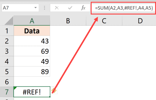
You can see that the third argument in the formula has become #REF! (which earlier referred to the cell that we deleted).
Take away / How to Fix: Before you delete any data that is being used in formulas, make sure there are no errors after the deletion. It’s also recommended that you create a backup of your work regularly to make sure you always have something to fall back on.
Incorrect Placement of Parenthesis (BODMAS)
As your formulas start to get bigger and more complex, it’s a good idea to use parenthesis to be absolutely clear of what part belongs together.
In some cases, you may have the parenthesis at the wrong place, which can either give you a wrong result or an error.
And in some cases, it’s recommended to uses parenthesis to make sure the formula understands what needs to be grouped and calculated first.
For example, suppose you have the following formula:
=5+10*50
In the above formula, the result is 505 as Excel first does the multiplication and then the addition (as there is an order of precedence when it comes to operators).
If you want it to first do the addition and then the multiplication, you need to use the below formula:
=(5+10)*50
In some cases, the order of precedence may work for you, but it’s still recommended that you use the parenthesis to avoid any confusion.
Also, in case you’re interested, below is the order of precedence for various operators often used in formulas:
| Operator | Description | Order of Precedence |
| : (colon) | Range | 1 |
| (single space) | Intersection | 2 |
| , (comma) | union | 3 |
| – | Negation (as in –1) | 4 |
| % | Percentage | 5 |
| ^ | Exponentiation | 6 |
| * and / | Multiplication & division | 7 |
| + and – | Addition & subtraction | 8 |
| & | Concatnenation | 9 |
| = < > <= >= <> | Comparison | 10 |
Take away / How to Fix: Always use parenthesis to avoid any confusion, even if you know the order of precedence and are using it correctly. Having parenthesis makes it easier to audit formulas.
Incorrect Use of Absolute/Relative Cell References
When you copy and paste formulas in Excel, it automatically adjusts the references. Sometimes, this is exactly what you want (mostly when you’re copy-pasting formulas down the column), and sometimes you don’t want this to happen.
An absolute reference is when you fix a cell reference (or range reference) so that it doesn’t change when you copy and paste formulas, and a relative reference is one that changes.
You can read more about absolute, relative, and mixed references here.
You may get an incorrect result in case you forget to change the reference to an absolute one (or vice versa). This is something that happens quite often to me when I am using lookup formulas.
Let me show you an example.
Below I have a dataset where I want to fetch the score in Exam 1 for the names in column E (a simple VLOOKUP use case)

Below is the formula that I use in cell F2 and then copies to all the cells below it:
=VLOOKUP(E2,A2:B6,2,0)

As you can see that this formula gives an error in some cases.
This happens because I haven’t locked the table array argument – it’s A2:B6 in cell F2, while it should have been $A$2:$B$6
By having these dollar signs before the row number and column alphabet in a cell reference, I am forcing Excel to keep these cell references fixed. So, even when I copy this formula down, the table array will continue to refer to A2:B6
Pro Tip: To convert a relative reference to an absolute one, select that cell reference within the cell, and press the F4 key. You would notice that it changes by adding the dollar signs. You can continue to press F4 until you get the reference you want.
Incorrect Reference to Sheet / Workbook Names
When you refer to other sheets or workbooks in a formula, you need to follow a specific format. And in case the format is incorrect, you will get an error.
For example, if I want to refer to cell A1 in Sheet2, the reference would be =Sheet2!A1 (where there is an exclamation sign after the sheet name)
And in case there are multiple words in the sheet name (let’s say it’s Example Data), the reference would be =’Example Data’!A1 (where the name is enclosed in single quotes followed by an exclamation sign).
In case you’re referring to an external workbook (let’s say you’re referring to cell A1 in ‘Example Sheet’ in the workbook named ‘Example Workbook’), the reference will be as shown below:
='[Example Workbook.xlsx]Example Sheet'!$A$1
And in case you close the workbook, the reference would change to include the entire path of the workbook (as shown below):
='C:\Users\sumit\Desktop\[Example Workbook.xlsx]Example Sheet'!$A$1
In case you end up changing the name of the workbook or the worksheet to which the formula refers to, it’s going to give you a #REF! error.
Also read: How to Find External Links and References in Excel
Circular References
A circular reference is when you refer (directly or indirectly) to the same cell where the formula is being calculated.
Below is a simple example, where I use the SUM formula in cell A4 while using it in the calculation itself.
=SUM(A1:A4)
Although Excel shows you a prompt letting you know about the circular reference, it will not do it for every instance. And this may give you the wrong result (without any warning).
In case you suspect circular reference in play, you can check which cells have it.
To do this, click the Formula tab and in the ‘Formula Auditing’ group, click on the Error Checking drop-down icon (the small downward pointing arrow).
Hover the cursor over the Circular reference option and it will show you the cell that has the circular reference issue.

Cells Formatted as Text
If you find yourself in a situation where as soon as you type the formula as hit enter, you see the formula instead of the value, it’s a clear case of the cell being formatted as text.

When a cell is formatted as text, it considers the formula as a text string and shows it as is.
It doesn’t force it to calculate and give the result.
And it has an easy fix.
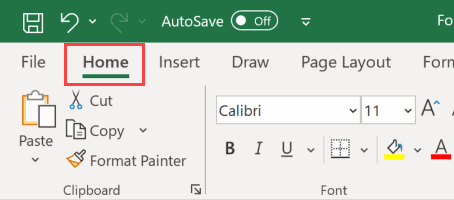
- Change the format to ‘General’ from ‘Text’ (it’s in Home tab in the Numbers group)
- Go to the cell that has the formula, get into the edit mode (use F2 or double click on the cell) and hit Enter
In case the above steps don’t solve the problem, another thing to check is whether the cell has an apostrophe at the beginning. A lot of people add an apostrophe to convert formulas and numbers to text.
If there is an apostrophe, you can simply remove it.
Text Automatically Getting Converted into Dates
Excel has this bad habit of converting that looks like a date into an actual date. For example, if you enter 1/1, Excel would convert it to 01-Jan of the current year.
In some cases, this may be exactly what you want, and in some cases, this may work against you.
And since Excel stores date and time values as numbers, as soon as you enter 1/1, it converts it into a number representing the January 1 of the current year. In my case, when I do this, it converts it into the number 43831 (for 01-01-2020).
This could mess with your formulas if you’re using these cells as an argument in a formula.
How to fix this?
Again, we don’t want Excel to automatically pick the format for us, so we need to clearly specify the format ourselves.
Below are the steps to change the format to text so that it doesn’t automatically convert text to dates:
- Select the cells/range where you want to change the format
- Click on the Home tab
- In the Number group, click on the Format drop-down
- Click on Text

Now, whenever you enter anything in the selected cells, it would be considered as text, and not changed automatically.
Note: The above steps would only work for data entered after the formatting has been changed. It will not change any text that has been converted to date before you made this formatting change.
Another example where this can be really frustrating is when you enter a text/number that has leading zeros. Excel automatically removes these leading zeros as it considers these useless. For example, if you enter 0001 in a cell, Excel will change it to 1. In case you want to keep these leading zeros, use the steps above.
Also read: Remove Formulas (but Keep Data) in Excel
Hidden Rows/Columns Can Give Unexpected Results
This is not a case of formula giving you the wrong result but of using the wrong formula.
For example, suppose you have a dataset as shown below and I want to get the sum of all the visible cells in column C.

In cell C12, I have used the SUM function to get the total sale value for all these given records.

So far so good!
Now, I apply a filter to the item column to only show the records for Printer sales.

And here is the problem – the formula in cell C12 still shows the same result – i.e., the sum of all the records.
As I said, the formula is not giving the wrong result. In fact, the SUM function is working just fine.
The issue is that we have used the wrong formula here.
SUM function can not account for the filtered data and give you the result for all the cells (hidden or visible). If you only want to get the sum/count/average of visible cells, use SUBTOTAL or AGGREGATE functions.
Key takeaway – Understand the correct use and limitations of a function in Excel.
These are some of the common causes that I have seen where your Excel formulas may not work or give unexpected or wrong results. I am sure there are many more reasons for an Excel formula to not work or update.
In case you know of any other reason (maybe something that irks you often), let me know in the comments section.
Hope you found this tutorial useful!
You may also like the following Excel tutorials:
- How to Lock Formulas in Excel
- How to Copy and Paste Formulas in Excel without Changing Cell References
- Show Formulas in Excel Instead of the Values
- Convert Text to Numbers in Excel
- Convert Date to Text in Excel
- Microsoft Excel Won’t Open; How to Fix it!
- Conditional Formatting Not Working in Excel
- Arrow Keys not Working in Excel | Moving Pages Instead of Cells
- 20 Advanced Excel Functions and Formulas


Hi Sumit,
I recognize these problems and have to deal with this a lot when I receive files or questions from other people. In most cases I can find the solution.
But I still have one very nasty problem, maybe you have a solution for this. I often have to use files with EAN-codes in it.
With use of the correct barcode fonts I can make these codes readable for scanners.
But the EAN-codes are automaticly transposed to Exponential values. Example: 8714632069985 is shown as 8,71463E+12 or 8,715E+12 in a smaller column.
I can change the cell properties to value without decimals or text but I hope there is a way I don’t have to change the cell properties because a lot of these files are imported from csv-files.
Very useful and interesting.
Thank you Summit.
Sumit,
Regarding your #REF! section, I have several hundred Excel files sent to me by others that may have #REF! errors due to cut/paste operations (which I have advised against) and the users don’t necessarily know it. I know I can find them in the opened file, but do you know how I can identify the “bad” files without opening them one at a time? Apparently, Windows File Explorer doesn’t recognize the #REF! text in the Excel file.
Thank you for the great tutorials,
Willie
When I format a cell with a custom format ;;; to make it unseen, the cell still counts as containing text, but when it is in a table, the filter drop down doesn’t show it. I have a column of check boxes that I would like to filter TRUE or FALSE without seeing the text, just the checked boxes. Making the text color match the background color works but is problematic with striped rows. Any suggestions?
never got it