
VLOOKUP Function – Introduction
VLOOKUP function is THE benchmark.
You know something in Excel if you know how to use the VLOOKUP function.
If you don’t, you better not list Excel as one of the strong areas in your resume.
I have been a part of the panel interviews where as soon as the candidate mentioned Excel as his area of expertise, the first thing asked was – you got it – the VLOOKUP function.
Now that we know how important this Excel function is, it makes sense to ace it completely to be able to proudly say – “I know a thing or two in Excel”.
This is going to be a massive VLOOKUP tutorial (by my standards).
I’ll cover everything there is to know about it, and then show you useful and practical VLOOKUP examples.
So buckle up.
It’s time for the takeoff.
When to use the VLOOKUP Function in Excel?
VLOOKUP function is best suited for situations when you are looking for a matching data point in a column, and when the matching data point is found, you go to the right in that row and fetch a value from a cell which is a specified number of columns to the right.
Let’s take a simple example here to understand when to use Vlookup in Excel.
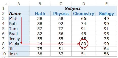
Remember when the exam score list was out and pasted on the notice board and everyone used to go crazy finding their names and their score (at least that’s what used to happen when I was in school).
Here is how it worked:
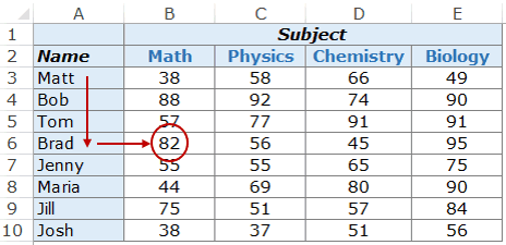
- You go up to the notice board and start looking for your name or enrolment number (running your finger from top to bottom in the list).
- As soon as you spot your name, you move your eyes to the right of the name/enrolment number to see your scores.
And that is exactly what the Excel VLOOKUP function does for you (feel free to use this example in your next interview).
VLOOKUP function looks for a specified value in a column (in the above example, it was your name) and when it finds the specified match, it returns a value in the same row (the marks you obtained).
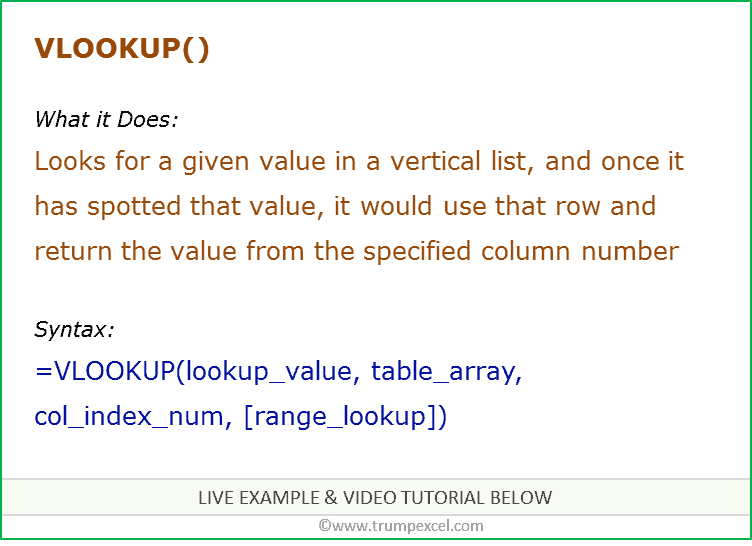
Syntax
=VLOOKUP(lookup_value, table_array, col_index_num, [range_lookup])
Input Arguments
- lookup_value – this is the look-up value you are trying to find in the left-most column of a table. It could be a value, a cell reference, or a text string. In the score sheet example, this would be your name.
- table_array – this is the table array in which you are looking for the value. This could be a reference to a range of cells or a named range. In the score sheet example, this would be the entire table that contains score for everyone for every subject
- col_index – this is the column index number from which you want to fetch the matching value. In the score sheet example, if you want the scores for Math (which is the first column in a table that contains the scores), you’d look in column 1. If you want the scores for Physics, you’d look in column 2.
- [range_lookup] – here you specify whether you want an exact match or an approximate match. If omitted, it defaults to TRUE – approximate match (see additional notes below).
Additional Notes (Boring, but important to know)
- The match could be exact (FALSE or 0 in range_lookup) or approximate (TRUE or 1).
- In approximate lookup, make sure that the list is sorted in ascending order (top to bottom), or else the result could be inaccurate.
- When range_lookup is TRUE (approximate lookup) and data is sorted in ascending order:
- If the VLOOKUP function can not find the value, it returns the largest value, which is less than the lookup_value.
- It returns a #N/A error if the lookup_value is smaller than the smallest value.
- If lookup_value is text, wildcard characters can be used (refer to the example below).
Now, hoping that you have a basic understanding of what the VLOOKUP function can do, let’s peel this onion and see some practical examples of the VLOOKUP function.
10 Excel VLOOKUP Examples (Basic & Advanced)
Here are 10 useful exampels of using Excel Vlookup that will show you how to use it in your day-to-day work.
Example 1 – Finding Brad’s Math Score
In the VLOOKUP example below, I have a list wth student names in the left-most column and marks in different subjects in columns B to E.
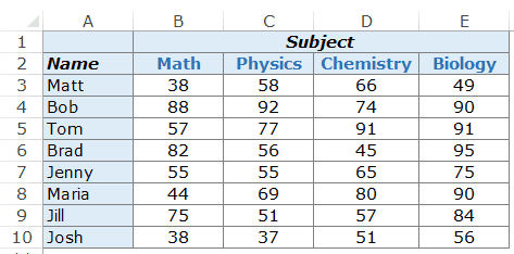
Now let’s get to work and use the VLOOKUP function for what it does best. From the above data, I need to know how much Brad scored in Math.
From the above data, I need to know how much Brad scored in Math.
Here is the VLOOKUP formula that will return Brad’s Math score:
=VLOOKUP("Brad",$A$3:$E$10,2,0)
The above formula has four arguments:
- “Brad: – this is the lookup value.
- $A$3:$E$10 – this is the range of cells in which we are looking. Remember that Excel looks for the lookup value in the left-most column. In this example, it would look for the name Brad in A3:A10 (which is the left-most column of the specified array).
- 2 – Once the function spots Brad’s name, it will go to the second column of the array, and return the value in the same row as that of Brad. The value 2 here indicated that we are looking for the score from the second column of the specified array.
- 0 – this tells the VLOOKUP function to only look for exact matches.
Here is how the VLOOKUP formula works in the above example.
First, it looks for the value Brad in the left-most column. It goes from top to bottom and finds the value in cell A6.
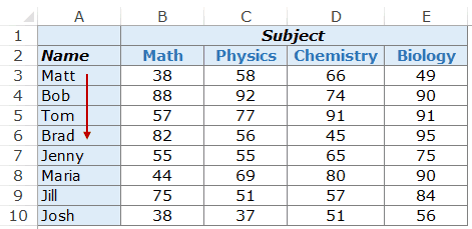
As soon as it finds the value, it goes to the right in the second column and fetches the value in it.
You can use the same formula construct to get anyone’s marks in any of the subjects.
For example, to find Maria’s marks in Chemistry, use the following VLOOKUP formula:
=VLOOKUP("Maria",$A$3:$E$10,4,0)
In the above example, the lookup value (student’s name) is entered in double quotes. You can also use a cell reference that contains the lookup value.
The benefit of using a cell reference is that it makes the formula dynamic.
For example, if you have a cell with a student’s name, and you are fetching the score for Math, the result would automatically update when you change the student’s name (as shown below):
If you enter a lookup value that is not found in the left-most column, it returns a #N/A error.
Example 2 – Two-Way Lookup
In Example 1 above, we hard-coded the column value. Hence, the formula would always return the score for Math as we have used 2 as the column index number.
But what if you want to make both the VLOOKUP value and the column index number dynamic. For example, as shown below, you can change either the student name or the subject name, and the VLOOKUP formula fetches the correct score. This is an example of a two-way VLOOKUP formula.
This is an example of a two-way VLOOKUP function.
To make this two-way lookup formula, you need to make the column dynamic as well. So when a user changes the subject, the formula automatically picks the correct column (2 in the case of Math, 3 in the case of Physics, as so on..).
To do this, you need to use the MATCH function as the column argument.
Here is the VLOOKUP formula that will do this:
=VLOOKUP(G4,$A$3:$E$10,MATCH(H3,$A$2:$E$2,0),0)
The above formula uses MATCH(H3,$A$2:$E$2,0) as the column number. MATCH function takes the subject name as the lookup value (in H3) and returns its position in A2:E2. Hence, if you use Math, it would return 2 as Math is found in B2 (which is the second cell in the specified array range).
Example 3 – Using Drop Down Lists as Lookup Values
In the above example, we have to manually enter the data. That could be time-consuming and error-prone, especially if you have a huge list of lookup values.
A good idea in such cases is to create a drop-down list of the lookup values (in this case, it could be student names and subjects) and then simply choose from the list.
Based on the selection, the formula would automatically update the result.
Something as shown below:
This makes a good dashboard component as you can have a huge data set with hundreds of students at the back end, but the end user (let’s say a teacher) can quickly get the marks of a student in a subject by simply making the selections from the drop down.
How to make this:
The VLOOKUP formula used in this case is the same used in Example 2.
=VLOOKUP(G4,$A$3:$E$10,MATCH(H3,$A$2:$E$2,0),0)
The lookup values have been converted into drop-down lists.
Here are the steps to create the drop down list:
- Select the cell in which you want the drop-down list. In this example, in G4, we want the student names.
- Go to Data –> Data Tools –> Data Validation.
- In the Data Validation Dialogue box, within the settings tab, select List from the Allow drop-down.
- In the source, select $A$3:$A$10
- Click OK.
Now you’ll have the drop-down list in cell G4. Similarly, you can create one in H3 for the subjects.
Example 4 – Three-way Lookup
What is a three-way lookup?
In Example 2, we’ve used one lookup table with scores for students in different subjects. This is an example of a two-way lookup as we use two variables to fetch the score (student’s name and the subject’s name).
Now, suppose in a year, a student has three different levels of exams, Unit Test, Midterm, and Final Examination (that’s what I had when I was a student).
A three-way lookup would be the ability to get a student’s marks for a specified subject from the specified level of exam.
Something as shown below:
In the above example, the VLOOKUP function can lookup in three different tables (Unit Test, Midterm, and Final Exam) and returns the score for the specified student in the specified subject.
Here is the formula used in cell H4:
=VLOOKUP(G4,CHOOSE(IF(H2="Unit Test",1,IF(H2="Midterm",2,3)),$A$3:$E$7,$A$11:$E$15,$A$19:$E$23),MATCH(H3,$A$2:$E$2,0),0)
This formula uses the CHOOSE function to make sure the right table is referred to. Let’s analyze the CHOOSE part of the formula:
CHOOSE(IF(H2=”Unit Test”,1,IF(H2=”Midterm”,2,3)),$A$3:$E$7,$A$11:$E$15,$A$19:$E$23)
The first argument of the formula is IF(H2=”Unit Test”,1,IF(H2=”Midterm”,2,3)), which checks the cell H2 and see what level of exam is being referred to. If it’s Unit Test, it returns $A$3:$E$7, which has the scores for Unit Test. If it’s Midterm, it returns $A$11:$E$15, else it returns $A$19:$E$23.
Doing this makes the VLOOKUP table array dynamic and hence makes it a three-way lookup.
Example 5 – Getting the Last Value from a List
You can create a VLOOKUP formula to get the last numerical value from a list.
The largest positive number that you can use in Excel is 9.99999999999999E+307. This also means that the largest lookup number in the VLOOKUP number is also the same.
I don’t think you would ever need any calculation involving such a large number. And that is exactly what we can use get the last number in a list.
Suppose you have a dataset (in A1:A14) as shown below and you want to get the last number in the list.
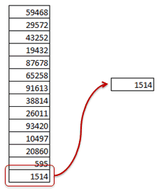
Here is the formula you can use:
=VLOOKUP(9.99999999999999E+307,$A$1:$A$14,TRUE)
Note that the formula above uses an approximate match VLOOKUP (notice TRUE at the end of the formula, instead of FALSE or 0). Also, note that the list doesn’t need to be sorted for this VLOOKUP formula to work.
Here is how the approximate VLOOKUP function works. It scans the left most column from top to bottom.
- If it finds an exact match, it returns that value.
- If it finds a value that is higher than the lookup value, it returns the value in the cell above it.
- If the lookup value is greater than all the values in the list, it returns the last value.
In the above example, the third scenario is at work.
Since 9.99999999999999E+307 is the largest number that can be used in Excel, when this is used as the lookup value, it returns the last number from the list.
In the same way, you can also use it to return the last text item from the list. Here is the formula that can do that:
=VLOOKUP("zzz",$A$1:$A$8,1,TRUE)
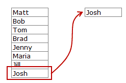
The same logic follows. Excel looks through all the names, and since zzz is considered bigger than any name/text starting with alphabets before zzz, it would return the last item from the list.
Example 6 – Partial Lookup using Wildcard Characters and VLOOKUP
Excel wildcard characters can be really helpful in many situations.
It’s that magic potion that gives your formulas super powers.
Partial look-up is needed when you have to look for a value in a list and there isn’t an exact match.
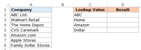
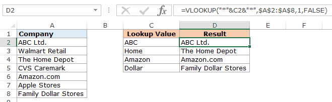
For example, suppose you have a data set as shown below, and you want to look for the company ABC in a list, but the list has ABC Ltd instead of ABC.
You can not use ABC as the lookup value as there is no exact match in column A. Approximate match also leads to erroneous results and it requires the list to be sorted in an ascending order.
However, you can use a wildcard character within the VLOOKUP function to get the match.
Enter the following formula in cell D2 and drag it to the other cells:
=VLOOKUP("*"&C2&"*",$A$2:$A$8,1,FALSE)
How does this formula work?
In the above formula, instead of using the lookup value as is, it is flanked on both sides with the wildcard character asterisk (*) – “*”&C2&”*”
An asterisk is a wildcard character in Excel and can represent any number of characters.
Using the asterisk on both sides of the lookup value tells Excel that it needs to look for any text that contains the word in C2. It could have any number of characters before or after the text in C2.
For example, cell C2 has ABC, so the VLOOKUP function looks through the names in A2:A8 and searches for ABC. It finds a match in cell A2, as it contains ABC in ABC Ltd. It doesn’t matter if there are any characters to the left or right of ABC. Until there is ABC in a text string, it will be considered a match.
Note: VLOOKUP function always returns the first matching value and stops looking further. So if you have ABC Ltd., and ABC Corporation in a list, it will return the first one and ignore the rest.
Example 7 – VLOOKUP Returning an Error Despite a Match in Lookup Value
It can drive you crazy when you see that there is a matching lookup value and the VLOOKUP function is returning an error.
For example, in the below case, there is a match (Matt), but the VLOOKUP function still returns an error.
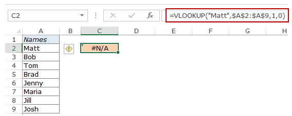
Now while we can see there is a match, what we can not see with a naked eye is that there could be leading or trailing spaces. If you have these additional spaces before, after, or in between the lookup values, it ISN’T an exact match.
This is often the case when you import data from a database or get it from someone else. These leading/trailing spaces have a tendency to sneak in.
The solution here is the TRIM function. It removes any leading or trailing spaces or extra spaces between words.
Here is the formula that’ll give you the right result.
=VLOOKUP("Matt",TRIM($A$2:$A$9),1,0)
Since this is an array formula, use Control + Shift + Enter instead of just Enter.
Another way could be to first treat your lookup array with the TRIM function to make sure all the additional spaces are gone, and then use the VLOOKUP function as usual.
Example 8 – Doing a Case Sensitive Lookup
By default, the lookup value in the VLOOKUP function is not case sensitive. For example, if your lookup value is MATT, matt, or Matt, it’s all the same for the VLOOKUP function. It’ll return the first matching value irrespective of the case.
But if you want to do a case-sensitive lookup, you need to use the EXACT function along with the VLOOKUP function.
Here is an example:
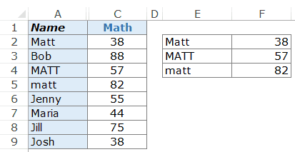
As you can see, there are three cells with the same name (in A2, A4, and A5) but with a different alphabet case. On the right, we have the three names (Matt, MATT, and matt) along with their scores in Math.
Now the VLOOKUP function is not equipped to handle case-sensitive lookup values. In this above example, it would always return 38, which is the score for Matt in A2.
To make it case sensitive, we need to use a helper column (as shown below):
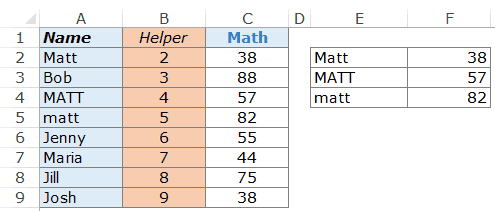
To get the values in the helper column, use the =ROW() function. It will simply get the row number in the cell.
Once you have the helper column, here is the formula that will give the case-sensitive lookup result.
=VLOOKUP(MAX(EXACT(E2,$A$2:$A$9)*(ROW($A$2:$A$9))),$B$2:$C$9,2,0)
Now let’s break down and understand what this does:
- EXACT(E2,$A$2:$A$9) – This part would compare the lookup value in E2 with all the values in A2:A9. It returns an array of TRUEs/FALSEs where TRUE is returned where there is an exact match. In this case, it would return the following array: {TRUE;FALSE;FALSE;FALSE;FALSE;FALSE;FALSE;FALSE}.
- EXACT(E2,$A$2:$A$9)*(ROW($A$2:$A$9) – This part multiplies the array of TRUEs/FALSEs with the row number. Wherever there is a TRUE, it gives the row number, else it gives 0. In this case, it would return {2;0;0;0;0;0;0;0}.
- MAX(EXACT(E2,$A$2:$A$9)*(ROW($A$2:$A$9))) – This part returns the maximum value from the array of numbers. In this case, it would return 2 (which is the row number where there is an exact match).
- Now we simply use this number as the lookup value and use the lookup array as B2:C9
Note: Since this is an array formula, use Control + Shift + Enter instead of just enter.
Example 9 – Using VLOOKUP with Multiple Criteria
Excel VLOOKUP function, in its basic form, can look for one lookup value and return the corresponding value from the specified row.
But often there is a need to use VLOOKUP in Excel with multiple criteria.
Suppose you have a data with students name, exam type, and the Math score (as shown below):
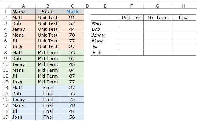
Using the VLOOKUP function to get the Math score for each student for respective exam levels could be a challenge.
For example, if you try using VLOOKUP with Matt as the lookup value, it’ll always return 91, which is the score for the first occurrence of Matt in the list. To get the score for Matt for each exam type (Unit Test, Mid Term and Final), you need to create a unique lookup value.
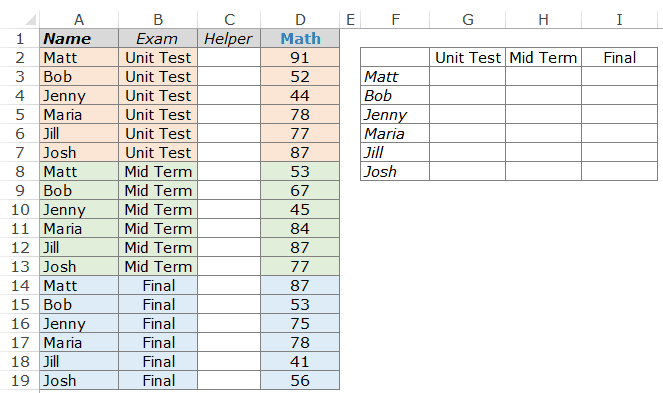
This can be done using the helper column. The first step is to insert a helper column to the left of the scores.
Now, to create a unique qualifier for each instance of the name, use the following formula in C2: =A2&”|”&B2
Copy this formula to all the cells in the helper column. This will create unique lookup values for each instance of a name (as shown below):
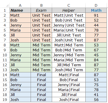
Now, while there were repetitions of the names, there is no repetition when the name is combined with the level of examination.
This makes it easy as now you can use the helper column values as the lookup values.
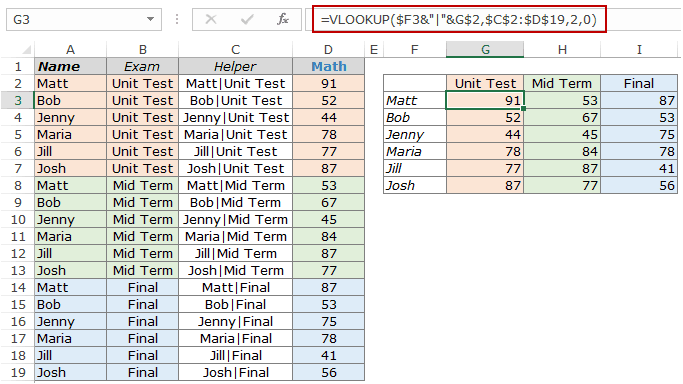
Here is the formula that’ll give you the result in G3:I8.
=VLOOKUP($F3&"|"&G$2,$C$2:$D$19,2,0)
Here we have combined the student name and the level of examination to get the lookup value, and we use this lookup value and checks it in the helper column to get the matching record.
Note: In the above example, we have used | as the separator while joining text in the helper column. In some exceptionally rare (but possible) conditions, you may have two criteria that are different but ends up giving the same result when combined. Here is an example:
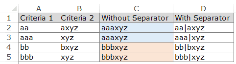
Note that while A2 and A3 are different and B2 and B3 are different, the combinations end up being the same. But if you use a separator, then even the combination would be different (D2 and D3).
Here is a tutorial on how to use VLOOKUP with multiple criteria without using helper columns. You can also watch my video tutorial here.
Example 10 – Handling Errors while Using the VLOOKUP Function
Excel VLOOKUP function returns an error when it can not find the specified lookup value. You may not want the ugly error value disturbing the aesthetics of your data in case VLOOKUP can’t find a value.
You can easily remove the error values with any meaning full text such as “Not Available” or “Not Found”.
For example, in the example below, when you try to find the score of Brad in the list, it returns an error as Brad’s name is not there in the list.
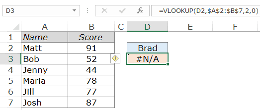
To remove this error and replace it with something meaningful, wrap your VLOOKUP function within the IFERROR function.
Here is the formula:
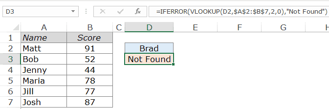
=IFERROR(VLOOKUP(D2,$A$2:$B$7,2,0),"Not Found")
The IFERROR function checks if the value returned by the first argument (which is the VLOOKUP function in this case) is an error or not. If it’s not an error, it returns the value by the VLOOKUP function, else it returns Not Found.
IFERROR function is available from Excel 2007 onwards. If you are using versions prior to that, use the following function:
=IF(ISERROR(VLOOKUP(D2,$A$2:$B$7,2,0)),"Not Found",VLOOKUP(D2,$A$2:$B$7,2,0))
Also See: How to handle VLOOKUP Errors in Excel.
That’s it in this VLOOKUP tutorial.
I’ve tried to cover major examples of using the Vlookup function in Excel. If you would like to see more examples added to this list, let me know in the comments section.
Note: I’ve tried my best to proofread this tutorial, but in case you find any errors or spelling mistakes, please let me know 🙂
Using VLOOKUP Function in Excel – Video
Related Excel Functions:
- Excel HLOOKUP Function.
- Excel XLOOKUP Function
- Excel INDEX Function.
- Excel INDIRECT Function.
- Excel MATCH Function.
- Excel OFFSET Function.
You May Also Like the Following Excel Tutorials:


Thanks a lot Sumit! I have seen many resources on vlook up, but your way is so simple to understand and also to help others understand. 🙂
can you please provide the excel sheet of above examples
Very helpful tutorial. Can anyone please guide how was the data validation drop down created in Example 4 for the Term exams (cell H2) done as it has multiple range areas which is not accepted in the simple ‘list’ function.
Thank you for this tutorial! I have tried a few video tutorials on youtube and step-by-step on other websites, but they did not successfully explain the way VLOOKUP actually works in the background, which was confusing to me.
This one is going from the core basics and building up on top of that which is how I prefer to understand and learn things!
I saw you mentioned to let you know if people notice some spelling errors so here is may take on that: The sentence “From the above data, I need to know how much Brad scored in Math.” is written twice in a row. 🙂
Thank you once again! Much appreciated!
So much love the teaching,o simplified. Thanks so much
hai summit,
very useful site, way of your teaching style is wonderful.
explaining with videos are so helpful and understandable .
Hi Sumit,
Can you provide me with the proper vlookup formula to use if pulling data from a separate worksheet in the same workbook? I can use the regular lookup function and it works but it’s pulling the wrong information. Here is the formula I’m using for lookup (=lookup(d9, Code!A2:A164,CodeE2:E164).
Hi Sumit,
Really your videos in Excel are very helpful and I need to learn many more techniques in Excel. How to automate the data from the previous Excel to the New Excel Book.
some new things even for experts
There must be an error in the Additional Notes section because its contradicting what is said in the 5th example: “If the VLOOKUP function can not find the value, it returns the *latest* value”, not greatest, “which is less than the lookup_value.”
Hello Nick.. The additional notes mention points when the data is sorted in ascending order. In that case, when VLOOKUP doesn’t find the value, it will give the largest value which is less than the lookup value.
In example 5, the data doesn’t need to be sorted and since we are looking for a really large number, it will go to the last cell and then return that last cell. This also work in case the data is sorted and it would then return the largest value.
Awesome , easiest way to learn & revise excel
Yes sir . I want to pick data such as : = Vlookup(C5, Vatlieu!$B$16:$B27,2,0) on the same workbook . Why it does’nt run ? Error : #Ref or #N/A . Can you help me . Very Thank .
Check your table array!!! It shows a
reference error. Akshay Magre
Example 4 – Three-way Lookup
Can I do for multi-sheet using same formula as per Example 4 but already tried is not coming, please find the way to do it
I have no word to thanks that you share by so easy method..
I request You to share the File with various way….
how to create dropdown list for 3 different tables headings?
how did you create the dropdown list for unit test, mid term, final in 3 way lookup function? please explain
Awesome!
Sorry
Good information @ mbaminiprojects.com
There are two columns of different numbers and I want to find out using a vlookup which numbers are missing
how to do left and right side Freeze pens in excel
Hi,
I have 2 worksheets. One reference number is common in both the sheets. I want to import data on one sheet. Only those entries which are not there, since I don’t need repetitive columns. When I put the formula it gives an error. I have tried with if error as well. It again returns “not found” for all the data. Need help.
Definitely need some type of excel document to go along with this training
Can you share the examples in excel please
For the three way how do we get data validation to work for the three titles since they come from three separate areas? I keep getting an error when I try to create a drop down list with data validation and pressing ctrl key for the three titles.
I created the list in separate cells and then formatted them to blend in with the background. From memory, I think data validation is found as ALT + A + V. Best of luck
ow it is so nice thank you
Won’t it be better if you attach the excel sheet which you used in these examples.
Without hands-on, it’s of no use.
I realize you were illustrating VLOOKUP techniques and your selection is very good. You could, however (also), use SUMPRODUCT for example 9 and avoid the helper column:
=SUMPRODUCT(($E2=$A$2:$A$19)*(F$1=$B$2:$B$19)*$C$2:$C$19)
Worked great!
Super Sumit Explanation are really superp I never miss your tutorial whenever it is posted on this blog. I always watch your turorial eagerly. Thanks.
Nicely explained
Great explanation. Can you share the examples as worksheets also ?
Very Good …. Learned some new things..
Advanced Excel Training Mumbai, Delhi, Gurgaon, Bangalore, Chennai. Excel Next offers training like MS Excel, MS Powerpoint, MS Excel VBA and many more.
Advanced Excel Training Gurgaon
I really like your post.It’s really informative and interesting.I really appreciate that.Thank you for sharing valuable information. Nice post. I enjoyed reading this post. The whole blog is very nice found some good stuff and good information here Thanks.
MS Excel
Hi Sumit,
Is it possible to apply VLOOKUP along with formats? I have a master sheet from where I need to copy data into another sheet, however the constraint is the reference columns have got some formats like date and time stamp, currency, etc. and I need to copy the details as is by applying VLOOKUP. To the best of my knowledge its not possible without applying VBA. Just wanted to check with you if you can give me a non VBA solution :).
I can’t think of any non-VBA method to do this!
Thanks for your prompt response! If I can ask for your assistance as in how can i perform the aforesaid action.
Q. क्या मैं हिंदी में प्रश्न पूछ सकता हूँ।
Hi, I completely understand your question. This was the same problem with me in excel.
And then I got a YouTube channel ( Learn With Lokesh Lalwani) I always learn everything about the excel this channel. I would like to suggest that you can also learn from this channel.
Thanks
Aap Vlookup ke bare me is youtube channel par sab kuch sikh sakte hai. or bhi kafi sare topics hai.
Great post. Most Excel users are still using VLOOKUP rather than INDEX/MATCH. So it’s great to see VLOOKUP being used in so many different ways (some of which I will definitely be learning from).
Good Tutorial.
Thanks for commenting.. Glad you liked it
I want to add, that VLOOKUP is able to look up from right to left also.
Hello Armen. . Yes, VLOOKUP can look to the left as well, but in such a case, I prefer using INDEX/MATCH formula combination
Thanks.
Hi Sumit, Would you please share an example on this
Excellent Tutorial. Learned a lot!
Thanks for commenting.. Glad you liked it!
Hi Sumit
Opened my eyes to vlookup
I have and do use it, and didn’t know as much as what you have explained
Good job
Thanks for commenting Rahul.. Glad you found the tutorial useful.
Very well explained! It saved me a lot of time!
Thanks Aanchal.. Glad you found this useful 🙂