Excel INDEX Function (Examples + Video)
When to use Excel INDEX Function
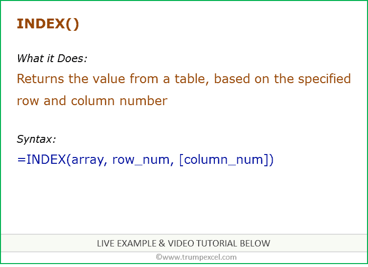
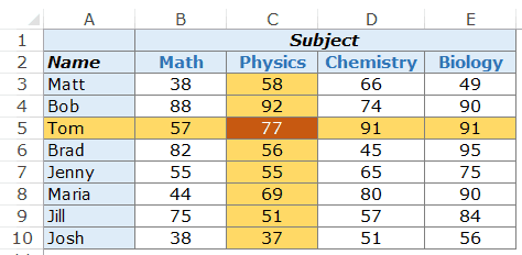
Excel INDEX function can be used when you want to fetch the value from a tabular data and you have the row number and column number of the data point. For example, in the example below, you can use the INDEX function to get the marks of ‘Tom’ in Physics when you know the row number and the column number in the data set.
What it Returns
It returns the value from a table for the specified row number and column number.
Syntax
=INDEX (array, row_num, [col_num])
=INDEX (array, row_num, [col_num], [area_num])
INDEX function has 2 syntax. The first one is used in most cases, however, in case of three-way lookups, the second one is used (covered in Example 5).
Input Arguments
- array – a range of cells or an array constant.
- row_num – the row number from which the value is to be fetched.
- [col_num] – the column number from which the value is to be fetched. Although this is an optional argument, but if row_num is not provided, it needs to be given.
- [area_num] – (Optional) If array argument is made up of multiple ranges, this number would be used to select the reference from all the ranges.
Additional Notes (Boring Stuff.. But Important to Know)
- If the row number or the column number is 0, it returns the values of the entire row or column respectively.
- If INDEX function is used in front of a cell reference (such as A1:) it returns a cell reference instead of a value (see examples below).
- Most widely used along with the MATCH function.
- Unlike VLOOKUP, INDEX function can return a value from the left of the lookup value.
- INDEX function have two forms – Array form and the Reference form
- ‘Array form’ is where you fetch a value based on row and column number from a given table.
- ‘Reference form’ is where there are multiple tables, and you use the area_num argument to select the table and then fetch a value within it using the row and column number (see live example below).
Excel INDEX Function – Examples
Here are six examples of using Excel INDEX Function.
Example 1 – Finding Tom’s Marks in Physics (a two-way lookup)
Suppose you have a dataset as shown below:

To find Tom’s marks in Physics, use the below formula:
=INDEX($B$3:$E$10,3,2)
This INDEX formula specifies the array as $B$3:$E$10 which has the marks for all the subjects. Then it uses the row number (3) and column number (2) to fetch Tom’s marks in Physics.
Example 2 – Making the LOOKUP Value Dynamic using MATCH Function
It may not always be possible to specify the row number and the column number manually. You may have a huge data set, or you may want to make it dynamic so that it automatically identifies the name and/or subject specified in cells and give the correct result.
Something as shown below:
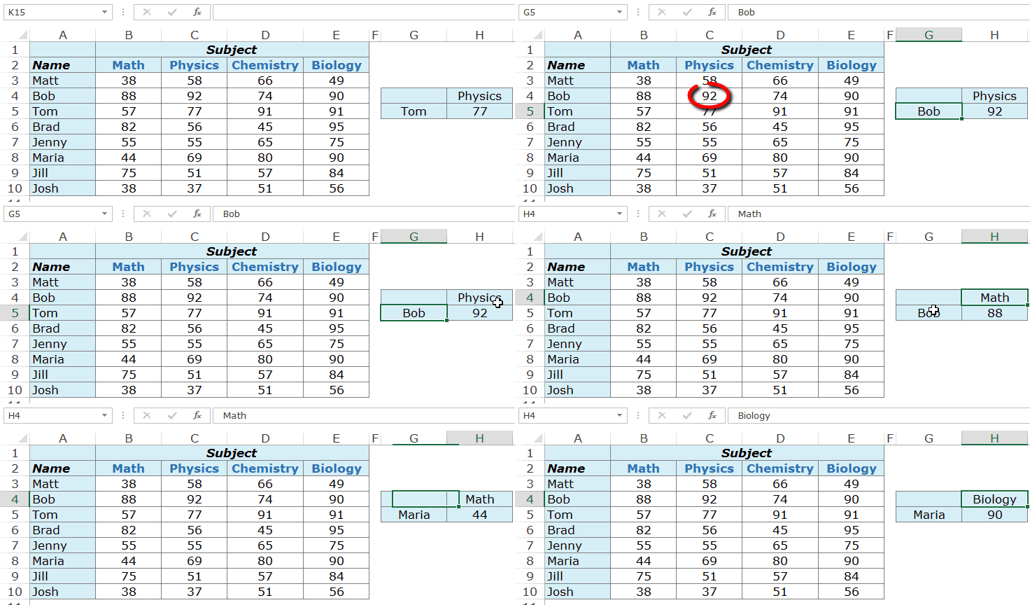
This can be done using a combination of the INDEX and the MATCH function.
Here is the formula that will make the lookup values dynamic:
=INDEX($B$3:$E$10,MATCH($G$5,$A$3:$A$10,0),MATCH($H$4,$B$2:$E$2,0))
In the above formula, instead of hard-coding the row number and the column number, MATCH function is used to make it dynamic.
- Dynamic Row Number is given by the following part of the formula – MATCH($G$5,$A$3:$A$10,0). It scans the name of students and identifies the lookup value ($G$5 in this case). It then returns the row number of the lookup value in the dataset. For example, if the lookup value is Matt, it’ll return 1, if it is Bob, it’ll return 2 and so on.
- Dynamic Column Number is given by the following part of the formula – MATCH($H$4,$B$2:$E$2,0). It scans the subject names and identifies the lookup value ($H$4 in this case). It then returns the column number of the lookup value in the dataset. For example, if the lookup value is Math, it’ll return 1, if it is Physics, it’ll return 2 and so on.
Example 3 – Using Drop Down Lists as Lookup Values
In the above example, we have to manually enter the data. That could be time-consuming and error-prone, especially if you have a huge list of lookup values.
A good idea in such cases is to create a drop down list of the lookup values (in this case, it could be student names and subjects) and then simply choose from the list. Based on the selection, the formula would automatically update the result.
Something as shown below:

This makes a good dashboard component as you can have a huge data set with hundreds of students at the back end, but the end user (let’s say a teacher) can quickly get the marks of a student in a subject by simply making the selections from the drop down.
How to make this:
The formula used in this case is the same used in Example 2.
=INDEX($B$3:$E$10,MATCH($G$5,$A$3:$A$10,0),MATCH($H$4,$B$2:$E$2,0))
The lookup values have been converted into drop-down lists.
Here are the steps to create the Excel drop down list:
- Select the cell in which you want the drop-down list. In this example, in G4, we want the student names.
- Go to Data –> Data Tools –> Data Validation.
- In the Data Validation Dialogue box, within the settings tab, select List from the Allow drop-down.
- In the source, select $A$3:$A$10
- Click OK.
Now you’ll have the drop-down list in cell G5. Similarly, you can create one in H4 for the subjects.
Example 4 – Return Values from an Entire Row/Column
In the above examples, we’ve used Excel INDEX function to do a 2-way lookup and get a single value.
Now, what if you want to get all the marks of a student. This can enable you to find the maximum/minimum score of that student, or the total marks scored in all subjects.
In simple English, you want to first get the entire row of scores for a student (let’s say Bob) and then within those values identify the highest score or the total of all the scores.
Here is the trick.
In Excel INDEX Function, when you enter the column number as 0, it will return the values of that entire row.
So the formula for this would be:
=INDEX($B$3:$E$10,MATCH($G$5,$A$3:$A$10,0),0)
Now this formula. if used as is, would return the #VALUE! error. While it displays the error, in the backend, it returns an array that has all the scores for Tom – {57,77,91,91}.
If you select the formula in the edit mode and press F9, you’ll be able to see the array it returns (as shown below):
Similarly, based on what the lookup value is, when the column number is specified as 0 (or is left blank), it returns all the values in the row for the lookup value
Now to calculate the total score obtained by Tom, we can simply use the above formula within the SUM function.
=SUM(INDEX($B$3:$E$10,MATCH($G$5,$A$3:$A$10,0),0))
On similar lines, to calculate the highest score, we can use MAX/LARGE and to calculate minimum, we can use MIN/SMALL.

Example 5 – Three Way Lookup Using INDEX/MATCH
Excel INDEX function is built to handle three-way lookups.
What is a three-way lookup?
In the above examples, we’ve used one table with scores for students in different subjects. This is an example of a two-way lookup as we use two variables to fetch the score (student’s name and the subject).
Now, suppose in a year, a student has three different levels of exams, Unit Test, Midterm, and Final Examination (that’s what I had when I was a student).
A three-way lookup would be the ability to get a student’s marks for a specified subject from the specified level of exam. This would make it a three-way lookup as there are three variables (student’s name, subject’s name, and the level of examination).
Here is an example of a three-way lookup:
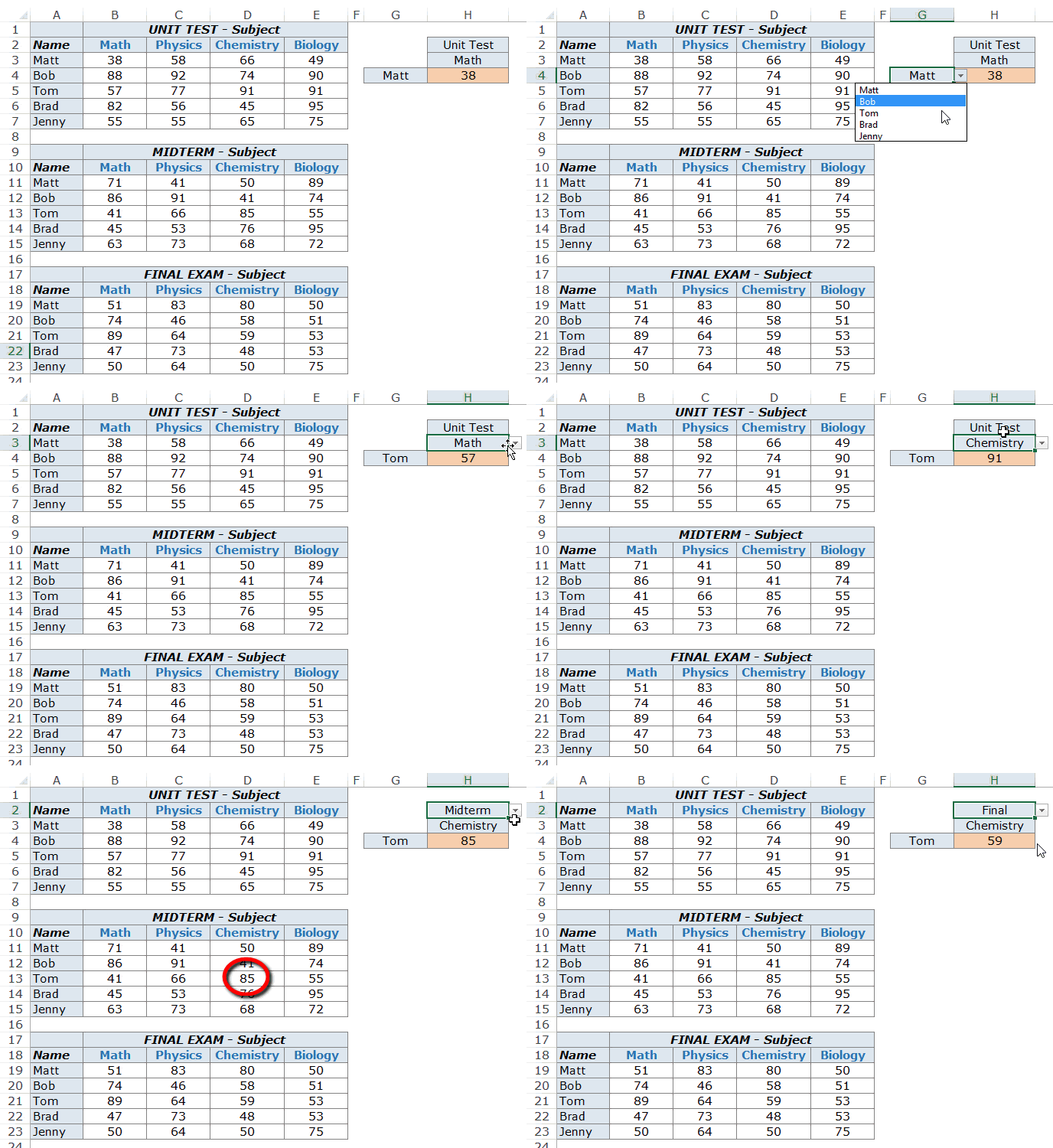
In the example above, apart from selecting the student’s name and subject name, you can also select the level of exam. Based on the level of exam, it returns the matching value from one of the three tables.
Here is the formula used in cell H4:
=INDEX(($B$3:$E$7,$B$11:$E$15,$B$19:$E$23),MATCH($G$4,$A$3:$A$7,0),MATCH($H$3,$B$2:$E$2,0),IF($H$2="Unit Test",1,IF($H$2="Midterm",2,3)))
Let’s break down this formula to understand how it works.
This formula takes four arguments. INDEX is one of those functions in Excel that has more than one syntax.
=INDEX (array, row_num, [col_num])
=INDEX (array, row_num, [col_num], [area_num])
So far in all the example above, we have used the first syntax, but to do a three-way lookup, we need to use the second syntax.
Now let’s see each part of the formula based on the second syntax.
- array – ($B$3:$E$7,$B$11:$E$15,$B$19:$E$23): Instead of using a single array, in this case, we have used three arrays within parenthesis.
- row_num – MATCH($G$4,$A$3:$A$7,0): MATCH function is used to find the position of the student’s name in cell $G$4 in the list of student’s name.
- col_num – MATCH($H$3,$B$2:$E$2,0): MATCH function is used to find the position of the subject name in cell $H$3 in the list of subject’s name.
- [area_num] – IF($H$2=”Unit Test”,1,IF($H$2=”Midterm”,2,3)): The area number value tells the INDEX function which array to select. In this example, we have three arrays in the first argument. If you select Unit Test from the drop-down, the IF function returns 1 and the INDEX functions select 1st array from the three arrays (which is $B$3:$E$7).
Example 6 – Creating a Reference Using the INDEX Function (Dynamic Named Ranges)
This is one wild use of the Excel INDEX function.
Let’s take a simple example.
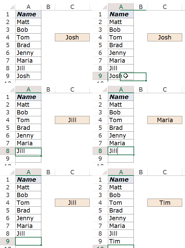
I have a list of names as shown below:

Now I can use a simple INDEX function to get the last name on the list.
Here is the formula:
=INDEX($A$2:$A$9,COUNTA($A$2:$A$9))
This function simply counts the number of cells that are not empty and returns the last item from this list (it works only when there are no blanks in the list).
Now, what here comes the magic.
If you put the formula in front of a cell reference, the formula would return a cell reference of the matching value (instead of the value itself).
=A2:INDEX($A$2:$A$9,COUNTA($A$2:$A$9))
You would expect the above formula to return =A2:”Josh” (where Josh is the last value in the list). However, it returns =A2:A9 and hence you get an array of names as shown below:
One practical example where this technique can be helpful is in creating dynamic named ranges.
That’s it in this tutorial. I’ve tried to cover major examples of using the Excel INDEX function. If you would like to see more examples added to this list, let me know in the comments section.
Note: I’ve tried my best to proof read this tutorial, but in case you find any errors or spelling mistakes, please let me know 🙂
Excel INDEX Function – Video Tutorial
Related Excel Functions:
- Excel VLOOKUP Function.
- Excel HLOOKUP Function.
- Excel INDIRECT Function.
- Excel MATCH Function.
- Excel OFFSET Function.
You May Also Like the Following Excel Tutorials:




your explanation is very clear and helpful.
I need many exercises for index and match functions
what is the practical use of Example 6?
Example 5 IS NOT WORKING… if you have a video explaining about Three Way Lookup Using INDEX/MATCH will be great..
Tried many times but it is showing error….
how can use index function to compare my student’s mark correct or not?
Thanks for your helpful resource. Please do option to download the practice sheet in this regard. That will helps easily particle on above mention examples.
hi
can you please help me in putting all non blank values from different column to one column.
i have values in 30 columns (coming by another formula – and changing each time) i wants to put all non blank values in one column (better if it ignore duplicate)
These resources are quite helpful
Thanks for the helpful resource. I ran across what seems like a bug in Excel’s INDEX() function, and am curious if others have run into this.
In the attached image, note how Excel’s treatment of a value of 0 for row or column depends on the location of the function. In call B3, a reference to row 1, col 0 results in an unexpected/unwanted result of 2 (the contents at row 1, column 2). In cell C1, a reference to row 0, col 1 results in an unexpected/unwanted result of 1 (the contents at row 1, column 1).
If, however, the same function calls are located outside of the row and column range of the array, the function returns #VALUE!, as expected, for an out of range reference. See cells D5 and E3, which are the exact same function calls as B3 and C1, respectively.
Is there any known reason why the function behaves differently depending on where it is placed relative to the target array? Is this behavior documented?
Thanks for any insight.
https://uploads.disquscdn.com/images/2b5614ecfaed959af45c64b066ab9d8e7ea330f1c6f4aaece611d6c9598005ab.jpg
=SUM(INDEX($B$3:$E$10,MATCH($G$5,$A$3:$A$10,0),0),1) , in this formula why did you use “,1” at the end.
Hey Deepak.. Thanks for pointing out.. It was a typo.. have corrected it.