Excel Skills (Basic, Intermediate, and Advanced)

Most Excel users learn how to use Excel In a fragmented way. They learn tidbits of Excel from various places, such as in-person training, written tutorials, or videos.

In this article, I wanted to create an overall structure that any Excel user can follow to enhance their basic, intermediate, or advanced Excel skills.

Given that there are so many things that one can use in Excel, I have divided this article into three sections – Basic Excel skills, Intermediate Excel Skills, and Advanced Excel skills.

Under each section, I have specified the things in Excel you can consider learning to become an Excel user of that specific level.

While it’s impossible for me to cover everything there is to learn in Excel, I have spent a lot of time structuring this article so that you know exactly the things you need to know if you want to get started with Excel (basic Excel skills) or and enhance your Excel skills (Intermediate/Advanced Excel skills).

Basic Excel Skills

Let’s look at some of the basic Excel skills you should know about that will get you started with Excel and also help you prepare for your next Excel interview.

If you are an Excel beginner and want to learn Excel from the start, you can check out my Free Excel Basic to Advanced Video Course (no sign-up needed)

Data Entry

While Excel has many advanced features and data analysis capabilities, the majority of people still use Excel as a record-keeping tool or a database tool.

So, if you are new to Excel, learning how to do proper data entry should be the first thing you should learn.

And it’s quite straightforward, to be honest.

You just select the cell where you want to do the data entry and then manually type the data.

And in case you want to enter a formula, you need to start with an equal sign (=) and then enter your formula.

Below are the data types that you can have in a cell in Excel:

• Text String – Anything which is not a number or a formula would be considered a text string (including alphanumeric strings, such as A123)
• Numbers
• Date/Time – While dates are stored as numbers in the back end of Excel, you can format the cell to show a number as a date or time.
• Formulas

When you enter anything in a cell in Excel and hit the Enter key, the entry is complete, and the cursor moves to the next line. And when you enter anything in a cell and then press the Escape key, the entry will be removed, and the cursor will stay on the same cell.

Cells / Rows / Columns Selection

Every Excel user must know how to properly select the cells, rows, or columns in the worksheet.

There’s hardly anything you can do in Excel without selecting the desired cells/range or objects in the worksheet.

When you click on a cell (or you use the arrow keys to select a cell), It becomes the active cell where you can do the data entry or formula entry.

You can also select multiple contiguous or noncontiguous cells. For example, if you select cell A1, hold the shift key, and then select cell B10, It is going to select all the cells in that range A1:B10

On the other hand, if you want to select noncontiguous cells, hold the control key and then make the selection.

For example, if you want to select cell A1 and B5, first select cell A1, then hold the Control key and then select B5.

You can also select one row or column, A contiguous range of rows/columns, or noncontiguous rows/columns.

Here is what you need to know about row/column selection:

• To select one specific row, click on the row label (a number) on the left side of the first cell in the row. Similarly, to select a specific column, click on the column label (a letter), just above the first cell in the column.

• To select multiple contiguous rows/columns, select the first row/column, hold the shift key, and then select the last row/columns

• To select multiple non-contiguous rows/columns, hold the Control key and then select the rows or the columns

Basic Shortcuts

Even though you can get started with Excel without using any shortcuts, I highly recommend you learn some basic Excel shortcuts.

Although Excel has a lot of keyboard shortcuts, here are some basic ones you can consider learning.

• Control + C – to copy a cell or range of cells
• Control + V – top paste copied cells
• Control + X – to cut a cell or range of cells
• Arrow keys – to move in the worksheet
• Escape – Cancels data entry and removes whatever you entered in the active cell.
• Control + S – to save the workbook
• Control + Z – to redo the past action
• F4 – to repeat the last action

Copy Pasting

You will need to know how to copy and paste data In Excel from the very first day you start using Microsoft Excel.

Below are some of the things you can do with copy-pasting in Excel:

• You can copy a cell and paste it anywhere else in the same worksheet, in another worksheet in the same workbook, or even in another workbook.
• You can copy a cell and paste it multiple times in the same workbook or a different one.
• You can copy and paste a contiguous or noncontiguous range of cells
• You can copy and paste objects and charts within Excel.

Basic Excel Functions

Excel has close to 500 functions, ranging from some very simple functions that take none or one/two arguments and inputs to some advanced complex functions that can be used to do a lot of different things.

Even if you are a beginner in Excel, I recommend you learn some of the basic Excel functions, such as:

• SUM – to get the sum of two or more values (or cells containing these values)
• COUNT – to get the count of cells that contain numbers
• IF – to check for a condition and return one value of the condition is true and return another value of the condition is false.
• AVERAGE – to get the average of two or more values
• AND / OR – To check whether the given set of conditions is true or not (AND returns TRUE if all the given conditions are met, and OR returns TRUE when one of the given conditions is true)

While you won’t need to learn all the Excel functions, as you get more comfortable using Excel, you can slowly learn other basic and more advanced Excel functions.

Inserting Notes in Cells (Previously Called Comments)

Excel allows you to add Notes to a cell in the worksheet.

This could be useful when you are going through your work in Excel, and you want to highlight and add some context to a cell or multiple cells.

Below is an example of a note that I have added to a cell:

To insert a note, simply right-click on the cell and then click on the ‘New Note’ option (or you can use the keyboard shortcut Shift + F2, where you need to hold the Shift key and press the F2 key to insert the note).

Once the note is inserted, a yellow box opens at the right of the cell, where you can enter the text you want in the note.

Note: In the prior versions of Excel, a Note used to be called a Comment. But this was changed in Excel and Microsoft 365, where a note is something that you insert for one cell, and a comment is something that can be like a conversation with a thread.

Delete Rows / Columns

As you start working with the data in Excel, one of the things you would be required to do is clean up your data by deleting some of the rows or columns.

You can select and delete individual rows or columns, or you can even select multiple contiguous or noncontiguous rows or columns and then delete them in one go.

To delete a single row, follow the below steps:

1. Right-click on any cell that you want to delete in a row.
2. Click on the Delete option
3. Select the ‘Entire row’ option
4. Click OK

The above steps would delete the row.

Similarly, you can also delete multiple rows by selecting multiple cells (which could be contiguous or noncontiguous, i.e., consecutive or non-consecutive), and then following the above steps.

Similarly, you can delete one or more columns by selecting the ‘Entire column’ option in Step #3.

In case you delete a row/column and then you want to get it back, you can undo that by using the shortcut Control + Z (hold the Control key and then press the Z key)

Insert Rows / Columns

Just like deleting rows and columns, you can also insert a row or a column in a specific location in the worksheet.

For example, if I want to insert a new column on the left of column E, I can follow the below steps:

1. Right-click on any cell in column E.
2. Click on the Insert option.
3. In the Insert dialog box that opens up, select the ‘Entire column’ option.
4. Click OK

The above steps would insert a new column which is on the left of column E.

Similarly, you can insert a new row by selecting the entire row option in Step #3.

Pro Tip: Excel is going to insert as many rows/columns as you have selected. For example, if I select cells D2 and E2, then right-click to open the Insert dialog box, and then select the ‘Entire column’ option, it will insert two columns to the left of column D. This is because I selected cells in two columns, to begin with.

Formatting

Excel has many different formatting options that will make your data look a lot better and improve readability.

Simple things such as making the headers bold, giving a border to the range of cells, filling color in some of the cells, changing the font size or the font type, specifying an alignment, etc., will make your data look much more professional and easier to peruse.

You can find most of the formatting options in the Font and Alignment group in the Home tab.

Below are the options that you can get in these two groups:

• Font Type
• Font Size
• Bold
• Italic
• Underline
• Border
• Fill Color
• Font Color
• Alignment Options
• Indent Options

Pro Tip: As you start working with Excel, you will realize that there are some formatting options that you use more than others. I recommend you learn the keyboard shortcuts to apply these formatting as it’ll help you get your work done a lot faster.

Data Filtering

Now that you know the basics of how to bring the data in Excel and how to copy-paste, rearrange, and format your data, let’s move to the next set of basic Excel skills – data analysis.

When you have a large data set in Excel, and you want to filter your data so that you only see a small subsection of that data, you can use the data filters option in Excel.

For example, if you have a data set for different states in the US, and you want to quickly filter your data so that you only see the data for New York, you can do that by applying a filter and filtering your data based on New York.

This way, only the data for New York is shown, and all the other records are hidden.

Let me show you how it works.

Below, I have a data set where I have the sales records for different sales reps that cater to different states, and I want to filter this data to only see the records for New York.

Below are the steps to do this:

1. Select any cell in the data set.
2. Click on the Data tab.
3. In the ‘Sort and Filter’ group, click on the ‘Filter’ icon. This will apply a filter to the data set, and you will see the filter drop-down icon in each cell in the header row.

4. Click on the filter dropdown icon for the State column.

5. Uncheck all the other options, and only keep the New York option checked.

6. Click OK

The above steps would instantly filter the data set to only show you the records that belong to New York, and all the other rows would be hidden.

This is a very simple example of using the filter in Excel, and I recommend you play with this feature to explore other options it has.

For example, you can filter a text-based column based on conditions such as whether it contains a specific string, it does not contain that string, or it starts or ends with that specific string, etc.

Similarly, if you have a column that contains numbers, you can use filter conditions such as filtering only those records where the number is equal to a specific value, it’s greater than or less than a specific value, or is in between a specific range.

Note: Excel allows you to alley multiple filters in your data set. For example, if you want to filter all the records where the state is New York and the sales value is more than 50,000, then you can apply two filters (one on the state column and one on the sales column)

Sorting

Another basic Excel skill you should learn is sorting in Excel.

Sorting allows you to quickly sort your data set based on the numeric value in the column or the text string.

For example, say I have a data set shown below where I have the sales rep name in column A, the state name in column B, and the sales value in column C.

With the sorting feature, I can rearrange the records so that the sales are in ascending order.

Below are the steps to sort the sales data from largest to smallest:

1. Select the entire data set
2. Click on the Data tab
3. In the Sort and Filter group, click on the Sort icon. This will open the Sort dialog box.

4. In the Sort dialog box, make sure the ‘My data has headers’ option is checked (in case it’s not checked already). We are doing this as our data set has headers, and we don’t want the headers to be sorted in the process.

5. Click on the sort by drop-down and then select the Sales option. Doing this ensures that the sorting is done based on the Sales column only.

6. Click on the Order drop-down and select ‘Largest to Smallest’

7. Click OK

Your data would instantly be sorted where the sales reps with the highest sales would be at the top, and the one at the lowest would be at the bottom.

In this example, I’ve sorted this data set based on only one column, but you can also sort based on multiple columns. I will cover multi-level sorting as part of the intermediate Excel skill section.

Remove Duplicates

Another useful data analysis tool you should master as part of your basic Excel skills is the ability to remove duplicates from your dataset.

Thankfully, an inbuilt feature in Excel allows you to quickly remove duplicates with a few clicks.

Below, I have a data set of names where there are repetitions.

Here are the steps to remove the names that are duplicates:

1. Select the entire data set from which you want to remove the duplicates
2. Click on the Data tab
3. In the ‘Data Tools’ group, click on the Remove Duplicate icon. This will open the ‘Remove Duplicates’ dialog box.

4. Check the ‘My data has header’ option if not checked already. You can uncheck this in case your data does not have a header cell/row.
5. Select the column name from which you want to remove the duplicates. In this case, we only have one column – Name.

4. Click Ok

As soon as you click OK, Excel removes all the duplicate names.

Note: In this example, I only had one column from which you wanted to remove the duplicates. In case you have a data set that spans across multiple columns, to use this feature, you would have to specify which columns should be considered to check for duplicates.

Wrap Text

Wrap text is a formatting feature that helps you in situations where the cell’s content is longer than the width of the cell.

In such situations, either the cell’s content would spill over and be shown in the next cell (which looks bad) or may get cut off, which means that the part that extends out of the cell would not be visible.

To tackle this issue, you can use the wrap text feature so that the cell’s content is wrapped within it and shown in multiple lines in the same cell.

Below, I have an idioms data set where the text in the cell is longer than the width of the cell and spills over to the adjacent cells.

Here are the steps to use wrap text on this data set:

1. Select the cells where you want to wrap the text
2. Click the Home tab
3. In the Alignment group, click on the Wrap Text icon.

As soon as you click on the Wrap Text icon, you will notice that the content in the cell has been rearranged so that it fits the width of the cell.

Note: The Wrap Text option works as a toggle, so when you click on it once, the wrap text format is applied to the selected cell, and when you click on it again, the wrap text format is removed.

Pro Tip: You can also use the keyboard shortcut ALT + H + W to apply wrap text to the selected cells. To use this shortcut, press these keys one after the other.

Find and Replace

As the name suggests, Find and Replace allows you to find a specific text string and replace it with another string.

To give you a very simple use case, suppose you have a list of URLs, and you want to remove the string ‘https://’ from these URLs. You can easily do that using find and replace (where you find ‘https://’ and replace it with a blank character)

Let me show you an example of how it works.

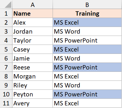
Below is a data set where I have employee names in column A and the training they have done in column B, and I want to replace the word MS with Microsoft.

Here are the steps to do this:

1. Select the cells in column B where you want to make the replacement.
2. Click the Home tab.
3. In the Editing group, click on the ‘Find & Select’ option
4. Click on the Replace option. This is going to open the Find and Replace dialog box

5. In the ‘Find what’ field, enter MS
6. In the ‘Replace with’ field, enter Microsoft

7. Click on Replace All

The above steps would replace the word MS with Microsoft.

You can also use the find and replace feature to find cells that contain a specific text string.

If you are a beginner, I recommend you play around with Find and Replace to get the hang of how it works. Once you know the basics, you can also learn about advanced uses of Find and Replace, such as using wild card characters or find formatting.

Pro Tip: You can use the keyboard shortcut Control + F to open the Find and Replace dialog box with the Find tab activated and Control + H to open the Find and Replace dialog box with the Replace tab activated

Basic Conditional Formatting

Conditional formatting is an amazing tool that allows you to format cells based on a given condition.

For example, If you have student scores data in Excel, you can use Conditional Formatting to highlight cells with scores above 80 and/or highlight cells with scores less than 35.

When you apply conditional formatting to a cell, it analyzes the value in that cell (or whatever condition you have used) and formats the cell if the condition is true or does nothing if the condition is false.

Conditional formatting has a lot of in-built conditions that you can access and use with a few clicks. Some examples include:

• Highlight cells that contain values that are greater than, less than, equal to, or in between a given range.
• Highlight cells that contain a specific text string.
• Highlight cells that contain dates that have occurred in the past one day, or past 7 days or the past month or in, the past year, etc.
• Highlight cells that contain duplicate values.
• Highlight cells that contain the top 10 or bottom 10 values, the top 10% or the bottom 10% values, or the values that are above average or below average.

Let me show you a simple example of how Conditional Formatting works in Excel.

I have a data set where I have the student’s name in column A and their score in column B, and I want to highlight cells where the score is more than 80.

Here are the steps to do this:

1. Select the range of cells that have those scores
2. Click the Home tab
3. In the Styles group, click on the Conditional Formatting option
4. Go to the ‘Highlight cell rules’ option and then click on ‘Greater than’. This will open the ‘Greater Than’ dialog box

5. Enter 80 in the first field

6. [Optional] Choose the formatting from the drop-down in which you want to highlight the cells
7. Click OK

The above steps would highlight all the cells with a score of more than 80 in the specified format.

As a beginner user learning basic Excel skills, I recommend you play with Conditional Formatting and learn how some of these inbuilt options work. Once you have mastered the basics of conditional formatting, you can then use it for more advanced use cases, such as highlighting every alternate row or highlighting cells based on values in another cell or column.

Basic Excel Charts

Excel offers a variety of charts that you can add to your worksheet with a few clicks, along with many basic and advanced customizations that can be done to the charts.

As an Excel beginner, it would be a good idea to learn how to create simple charts such as line charts, column charts, or bar charts.

Once you know how to insert these charts in the worksheet, you can also look at some basic customizations such as adding data labels, Customizing the access labels, adding a chart title, changing the color of the line or the bars, etc.

Also read: How to Describe Excel Skills in a Resume?

Intermediate Excel Skills

Now that I have covered a lot of basic Excel skills that you should know, here are some of the intermediate Excel skills you can learn to become more proficient in Excel.

Some of the features I cover in this section are already covered in the Basic Excel Skills section, and here I will be showing you an advanced level of usage for the same features (such as Sort or Filter options).

Freeze Panes

When you start working with large datasets in Excel, one problem you would face is that the headers of the data set disappear when you scroll down or scroll to the right.

Freeze pains allow you to make sure that the header rows or header columns are always visible while you are scrolling away in the worksheet.

Below are the steps to freeze the top row in your worksheet:

1. Click the ‘View’ tab
2. In the ‘Window’ Group, click on the ‘Freeze Panes’ option
3. In the options that show up, click on the ‘Freeze Top Row’ option.

The above steps would freeze the top row so that when you scroll down, that top row will always be visible.

Similarly, you can also freeze the left-most column as well as any number of top rows and left-most columns (for example, you can freeze and lock the top two rows and the three leftmost columns if you want).

Flash Fill

Flash Fill is an amazing tool that was introduced in Excel 2013.

It’s most useful in situations where you have data set in a column and you want to extract or modify that data by following a specific pattern.

For example, if I have full names (that would have a first name and a last name) in a column, and I want to extract the first name in the adjacent column, I can use Flash Fill to do that.

Let me show you how it works.

Below is a data set where I have the full name and column A, and I want to extract the first name only in the adjacent column.

Here are the steps to do this:

1. Enter the first expected result you want in cell B2. In this example, I would enter the name Michael in cell B2.

2. Select cell B3
3. Hold the Control key and press the E key. Alternatively, you can also go to the Home tab, and in the Editing group, click on the Fill option, and then click on the Flash Fill icon that appears in the drop-down.

When you do the above steps, Flash Fill will recognize that you are trying to extract only the first name from column A and give you the result in column B.

While I’ve shown you just one example of using Flash Fill, you can use it with any data set where there is an easily recognizable pattern that Flash Fill can understand and use to manipulate the data.

Note: It’s possible that Flash Fill may not be able to recognize the right pattern with just one result. In such cases in such cases, you can give three or four expected result entries in the adjacent column and then use Flash Fill.

Filter by Color

While I covered the filter feature as one of the basic Excel skills, it also has an advanced use where you can filter your data set based on the color of the cells.

Below, I have a dataset where I have some cells that are highlighted in blue color in column B, and I want to filter these records.

Here are the steps to do this:

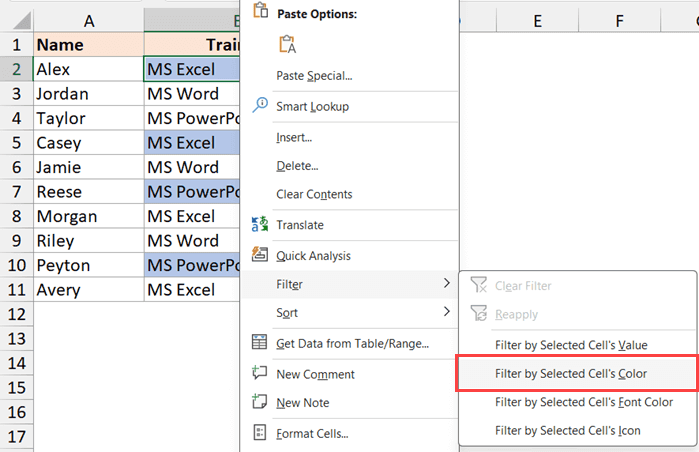
1. Right-click on any of the cells that have the color based on which you want to filter
2. Go to the Filter option
3. Click on the ‘Filter by Selected Cell’s Color’ option.

As soon as you follow the above steps, the data will be filtered, and only those records will be shown where the cells are in blue color in column B.

Note: Other similar options available to you are ‘Filter by Selected Cell’s Value’, ‘Filter by Selected Cell’s Font Color’, and ‘Filter by Selected Cell’s Icon’

Drop-Down Lists

A drop-down list is an interactive feature that allows you to get a list of options in a cell that you can choose from.

It can be quite useful when creating data entry forms.

It allows you to restrict the data that can be entered in a cell and also presents errors as the user can select from a pre-populated list instead of manually entering the data.

Drop-down lists are also very useful when you are creating dashboards that can quickly update as soon as you change the selection in the cell.

For example, you can have various charts showing the performance of each region, and these charts can automatically update as soon as you choose a different region from the drop-down.

Multi-level Sorting

I covered sorting a column as one of the Basic Excel Skills. And if you know how to do multiple-column sorting, you can add it to your collection of intermediate Excel skills.

When you do a multiple-column sorting, you need to specify the column that should be sorted first and then the next column (or columns) that should be sorted.

Let me show you how it works with an example.

Below, I have a dataset where I have the sales rep’s name, their region, and their sales values.

I now want to sort this data so that I have the records for the same regions together, and then within each region, the sales values should be sorted based on the value.

Here are the steps to do this:

1. Select any cell in the dataset (or select the entire dataset)
2. Click the Data tab
3. In the Sort & Filter group, click on the Sort icon. This will open the Sort dialog box.

4. Make sure the ‘My data has headers’ option is checked.
5. Click on the Sort by drop-down and then select the ‘Region’ option.
6. [Optional] Set the Sort Order (default is A to Z, and you can change it to Z to A if you want)

4. Click on the Add Level button. When you do this, it will add another level of sorting you can use.

4. Select ‘Sales’ from the Then by drop-down
5. Change the Sort Order from Largest to Smallest.

4. Click OK

The above steps would do the multiple-column sort, where first, the region column is sorted so that all records for Asia are together and all records for the US are together.

It then sorts based on the Sales values within each region group. So you get sales values in descending order for Asia as well as the US.

Using Formulas Conditional Formatting

I covered the in-built conditional formatting features as part of the basic Excel skills (such as highlighting values greater than or less than a specific value or the top 10 values of the top 10% values in a column).

Apart from these inbuilt features, Conditional Formatting also allows you to use custom formulas that can be used to highlight the cells.

This enables us to do a lot more advanced things with conditional formattings, such as highlight every second or every third or every nth row, highlight cells based on the value in another cell, highlight an entire row when a condition is met with one cell in that row, and a lot more.

Named Range

You already know that every cell in Excel has a reference, such as A1, B2, XF11, etc.

What a Named Range allows you to do is give a descriptive name to a cell or range of cells that can then be used in formulas instead of the reference.

It’s like giving your house an actual name instead of the entire address (which makes it a lot easier to remember the name and refer to it).

Imagine you’re working with a large dataset and need to refer to certain cells frequently. Instead of remembering “A2:A20,” you can name that range “MonthlySales.” It’s way easier to remember and work with.

Creating a Named Range

1. Select Cells: First, click and drag to highlight the cells you want to name.
2. Name Box: Look for the “Name Box” in the top-left corner. It usually shows the address of the active cell.
3. Enter Name: Click in the “Name Box,” delete the existing address, and type your custom name. Press Enter.

That’s it! You’ve just created a named range, and it can now be used anywhere in the workbook.

Naming Rules to Keep in mind when creating Named Ranges

1. No Spaces: Your name can’t have spaces. Use underscores or just smash the words together, like “MonthlySales.”
2. Unique Names: Each named range has to be unique. You can’t have two named ranges with the same name.
3. Start with a Letter: Names must start with a letter or an underscore. You can’t start a named range name with a number

Using Named Ranges in Formulas

Once you’ve named a range, you can use it in formulas. For example, instead of =SUM(A2:A20), you can now write =SUM(MonthlySales). Isn’t that easier to read and understand?

If you want to edit or delete your named ranges, go to the “Formulas” tab and click on “Name Manager.” Here, you can see all the named ranges and even change the cells they refer to.

Dynamic Named Ranges – I’m diving a bit deeper here, but stick with me. You can create “Dynamic Named Ranges” that automatically expand or shrink using Excel functions like OFFSET and COUNTA. This is super useful when your data range keeps changing. You can read my other article on creating dynamic named ranges here.

Excel Table

Excel table feature is another one of those fantastic tools that makes life so much easier when you’re handling data.

An Excel table is essentially a way to organize your data into a structured format. It’s not just about making it look pretty; it actually makes your data smarter and more manageable. Think of it like turning a simple range of cells into a mini database.

Once you know how Excel Tables work, there is no reason not to use these whenever you are working with data tables. In almost all cases, it is always a good idea to convert your data into an Excel table.

Why Use Excel Tables?

1. Easy Sorting & Filtering: With tables, you get dropdown arrows for sorting and filtering right at the top of each column.
2. Structured Referencing: One of the coolest things is how you can refer to table elements by their name. So instead of saying A1:A10, you can say [ColumnName]. It makes formulas way more readable and easier to understand. And you don’t need to remember the column names. You can get an intellisense drop-down that will show you the table name and all the column names in that table.
3. Auto-Fill Formulas: Add a formula in one cell, and it auto-fills down the whole column. It saves a ton of time and reduces errors. You don’t have to drag the fill handle every time you add new data.
4. Dynamic Ranges: When you add or remove data, Excel automatically updates the table range. Your formulas, charts, and pivot tables linked to the table update as well. You’re basically future-proofing your worksheet.
5. Readability: Alternate row colors (also called “banded rows”) make your table easier to read.
6. Total Row: This feature is a quick win for basic data analysis. It lets you add totals, averages, counts, and other calculations with just a few clicks. It’s all dynamic, too. Add more data, and the totals update automatically.
7. Slicers to Slice and Dice Your Data: Slicers is an amazing feature that allows you to filter your data with a few clicks. For example, if you have country-wise data you can insert a slicer that will show you all the country names, and you can quickly filter your data based on one or more countries. I use it quite often when creating interactive dashboards and reports (it looks pretty cool)

How to Create an Excel Table

1. Select Your Data: Highlight the range you want to turn into a table. Make sure it includes the headers.
2. Insert Table: Go to the Insert tab and then click on the Table option, or use the keyboard shortcut Ctrl + T (hold the control key and then press the T key).
3. Confirm Range: A dialog box will appear to confirm the data range. Check the box for “My table has headers” if your range includes headers. Click OK.

Boom, you’ve got a table!

Using Table References in Formulas

This is super cool. Once you’ve got a table, you can use structured references in your formulas.

Let’s say your table is named “SalesData” and you have a column labeled “Revenue.”

Instead of typing =SUM(B2:B10), you can write =SUM(SalesData[Revenue]). It’s much easier to understand, right?

Note: Now, if you go back to your Excel Table and add or delete some rows of data, you don’t need to worry about the formula, as it will automatically update.

Adding or Removing Rows and Columns

To add a row, simply click on the last cell in the last row and press Tab.

To add a column, type a new header in the column right next to your existing table. Excel will automatically extend the table for you.

To delete, right-click on the row or column header and select Delete Row or Delete Column.

Table Styles

Want to jazz up your table? Go to the Table Design tab that appears when you click on your table.

You’ll find options for different styles and colors there.

If you ever want to revert your table back to a regular range, go to the Table Design tab and click Convert to Range.

Also read: How to Remove Table Formatting in Excel?

Sparklines

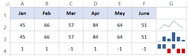
Sparklines are mini-charts that fit into a single cell. They’re used to display trends over time, like sales data, temperature, or stock prices.

Imagine you’ve got monthly sales data in a row, and you want a visual clue of how you’re doing.

Instead of creating a separate chart, you can place a Sparkline right next to your data to get the gist at a glance.

You can find the Sparklines option in the insert tab in the ribbon.

To insert a sparkline:

1. Select the cells that contain the data you want to visualize.
2. Click on the “Insert” tab.
3. In the Sparklines group, you’ll see options for Line, Column, and Win/Loss. Pick the one that suits you best.
4. A box will pop up asking where you’d like to place your Sparkline. Select a cell, and voila!

While Sparklines does not offer you as many customization options as a full-blown chart, there are still a lot of different customizations that you can do to the Sparklines.

For example, you can change the color of the lines, customize the axis, highlight the highest or lowest points, etc.

Intermediate Excel Functions

Now, let me cover some intermediate Excel functions. Each of these can be a game-changer once you get the hang of them.

XLOOKUP / VLOOKUP / HLOOKUP

First up is XLOOKUP.

XLOOKUP is a new function in Microsoft Excel for 365 and Excel on the Web. It’s like VLOOKUP without all the limitations (for example, if can lookup and fetch value from the left of the lookup column, which VLOOKUP can’t).

It lets you search a column for a specific value and then returns a value in the same row but from another column. It is very handy for pulling related data, like matching names with phone numbers.

If you don’t have XLOOKUP, you should definitely get comfortable using VLOOKUP (where V stands for Vertical Lookup)

Its cousin, HLOOKUP, does the same thing but horizontally. So you’re looking across rows instead of down columns. It is useful if your data is organized that way.

INDEX-MATCH

Another dynamic duo is INDEX and MATCH. They can be used separately but are most powerful when combined.

INDEX-MATCH is like VLOOKUP but more flexible. You can look both vertically and horizontally.

Also read: VLOOKUP Vs. INDEX/MATCH – Which One is Better? (Answered)

SUMIFS and COUNTIFS

These are useful in situations when you have complex conditions for summing or counting data.

SUMIFS function lets you sum data that meets multiple criteria, and COUNTIFS does the same for counting.

For example, if you have sales data and you only want to get the sum of all the sales values within a particular date range, you can use the SUMIFS function

CONCATENATE / CONCAT / TEXTJOIN

These functions help you join different strings of text.

Using these functions, you can quickly combine two or more cells or columns and get the result in one single cell/column.

TEXTJOIN is especially useful as it can join a range of cells and even include a delimiter. However, it’s a new function and is only available in Excel version 2019 and above (including Excel for Microsoft 365 and Excel for the Web)

Also read: CONCATENATE Excel Range (with and without separator)

TEXTSPLIT, TEXTBEFORE, TEXTAFTER

For text manipulation, these are your friends. These are new functions available in Excel for Microsoft 365, and I can’t tell you how happy I am that these functions are now available.

There are so many text manipulation things you can do with these functions that used to take a lot of time, and formula gymnastics earlier.

For example, if you quickly want to split the content of a cell into multiple columns or multiple rows based on 1 or 2 delimiters, you can easily do that using the TEXTSPLIT function. This used to be a long and complex earlier.

Similarly, if you want to extract the text before or after a specific delimiter or text string, you can do that using the TEXTBEFORE or TEXTAFTER function.

REPLACE / SUBSTITUTE

The names are quite self-explanatory.

The REPLACE function allows you to replace part of a text string with another string. It’s precise because you specify the exact start position and length of the text you want to replace.

The SUBSTITUTE function is a bit different but also super handy. It replaces occurrences of a specific substring within a text string with another string.

In most cases, these functions are used in conjunction with other functions to achieve complex text manipulation.

FILTER / SORT

Till a few years ago, filtering and sorting your data was done using the dedicated filter and sort functionality in Excel.

While these are pretty useful, having a dedicated FILTER and SORT function makes it a lot easier now to manipulate and rearrange data.

For example, if I have the sales records for multiple sales reps in different countries, I can use the FILTER function to give me only the sales records for the United States or filter the get records for the US and UK only.

You can check my detailed article on using the FILTER function.

Similarly, you can use the SORT function to easily sort the data right there in the worksheet with a simple formula.

One big benefit of having these formulas is that it makes the result dynamic, which means that in case your original data changes, the result of FILTER function or the SORT function would automatically update

OFFSET

The OFFSET function is a bit advanced but very powerful. It allows you to refer to a cell that has a specific number of rows and columns away from another cell.

While it’s not commonly used, it can be a lifesaver when you’re trying to achieve complex tasks.

These are some of the intermediate Excel functions that I’ve covered in this section. Some other functions that you can also look at can be:

• IFERROR
• IMAGE
• UNIQUE
• SUMPRODUCT
• WORKDAY / NETWORKDAYS

Excel Themes

Whenever you open Excel, you are using the default theme in Excel called Office.

It’s this theme that determines what font or colors should be used. For example, when you insert the bar chart, the bars will be blue in color (as that’s what’s coded in the theme).

You can easily change the theme so that the default settings can be changed.

So, if you want the default font to be Calibri instead of Aptos, and the chart colors to be red instead of bleu, you can do that by editing the theme (or choosing from the pre-made themes if that suits your need)

Here’s why you might want to switch up themes in Excel:

Consistent Colors and Styles

Changing a theme applies a uniform style across all elements of your workbook.

This means your charts, tables, and text all have matching colors and fonts, making everything look integrated and professional.

Most medium and large-size companies have their brand guidelines, and you can easily customize the theme so that every time you open a new Excel file, it already has those brand colors/font/styles integrated into it.

Enhanced Readability

Themes are designed with readability in mind.

The font pairings and color contrasts are chosen to make the data and text easier to read, which can be crucial when you’re sharing the workbook with others.

Time-Saving

If you always customize your worksheet so it has a specific set of colors/fonts that are used, you can create a theme and use that in every workbook you open. This can be a huge time saver.

For example, in one of the consulting companies I worked in at the beginning of my career, we had different color schemes we needed to follow for different clients.

So, I created separate Excel themes that used the client-specified colors and fonts. This one-time effort saved me and my team a lot of time (and time equals money in consulting)

Update the Theme Instead of Updating Each Element

Need to change the color of bars in the charts or font midway through a project?

Instead of editing each element individually, just edit the theme, and all the associated elements will update automatically.

Hyperlinks

Hyperlinks in Excel are useful when you want the user to have the ability to click on a link and navigate to some cell/range in the same worksheet/workbook or even other open workbooks.

You can also create hyperlinks that will take the user to a webpage or open a file saved on your system or shared drive.

Why Use Hyperlinks?

1. Navigating Large Workbooks: Makes moving around large workbooks easier.
2. Better Organization: Helps keep related data and files interconnected. For example, if you have created a summary table, you can create a hyperlink that will take the user to the source data.
3. User-Friendly: Makes it easier for people who aren’t familiar with your workbook to find what they need. I use this when creating dashboards where I often link to sheets that have instructions on how to use the dashboard.
4. Access to External References: Quickly access web resources or external files related to your data.

Types of Hyperlinks in Excel

1. Cell References: Use it to jump to another part of the same or different worksheet. Super handy for large files.
2. Web Page: You can create a hyperlink to a webpage in a cell. Clicking the link opens the website in your default web browser.
3. Email: You can link to an email address. Clicking it will open your default email client with that email address filled in.
4. File: You can link to other files on your computer. Clicking the hyperlink will open that file.

When you enter a URL or email in a cell in Excel and hit the Enter key, it automatically converts it into a hyperlink

There are two ways to create a hyperlink in Excel:

• Using the Insert Link option, which is available in the Insert tab in the ribbon
• Using the Hyperlink function

Using Wild Cards Characters in Excel

Once you learn how to use Wild card characters in Excel, you can confidently call yourself an intermediate/advanced Excel user. It’s not hard to learn how this works, but I can assure you it will make you look like an Excel magician.

Wildcards in Excel help you find what you’re looking for when you only have partial information.

There are mainly three wildcards: the asterisk (*), the question mark (?), and the tilde (~).

The Asterisk (*)

This is the most versatile (and the one that’s most used).

It can represent any number of characters in a string. For example, if you search for “Ex*,” Excel would match “Excel,” “Example,” and even “Extravagant.”

The Question Mark (?)

This one stands in for a single character. So if you search for “Te?t,” Excel would find “Text” and “Tent,” but not “Treat.”

The Tilde (~)

This is the escape character. Use it when you actually want to search for an asterisk, question mark, or tilde. Just put it right before the character you’re searching for, like “~*”.

Where to Use Wildcards in Excel

1. Searching: You can use wildcards in the Find and Replace dialog box.
2. Filtering: When filtering data, you can use wildcards in the criteria field to filter records that fit the wildcard pattern. For example, I can use the filter criteria *Excel* to filter any cell that contains the word Excel.
3. Formulas: Wildcards are often used in functions like XLOOKUP/VLOOKUP, HLOOKUP, MATCH, and SEARCH to make the search criteria more flexible.

Below is a video where I show some examples of using wildcard characters in Excel:

Pivot Table

Pivot tables have a separate fan base in the Excel world.

If you go and survey Excel fans, I’m sure you’ll find that most people are raving fans of Pivot Tables.

The level of summarization and analysis that can be done by simple drag and drop in Pivot tables is nothing short of magic.

What Is a Pivot Table, You Ask?

A Pivot Table helps you summarize and analyze large datasets. Imagine you have rows upon rows of sales data.

With a Pivot Table, you can easily find out, say, the total sales for each product. or total sales by region (or region and sales rep).

There is no way I can tell you everything or even enough about using Pivot Tables in this one single article.

Here are some Pivot Table articles that you can read:

• Creating a Pivot Table in Excel
• Preparing Source Data For Pivot Table
• How to Filter Data in a Pivot Table in Excel
• How to Group Dates in Pivot Tables in Excel
• How to Refresh Pivot Table in Excel
• Delete a Pivot Table in Excel
• Move a Pivot Table to a Different Worksheet or Workbook

Printing Your Excel Work

If you need to print your Excel work, you’ll find enough in-built printing options to cater to almost all your needs.

In the Page Layout tab in the ribbon, you will find many print-related options, such as:

• Setting the margins of the document that would be printed
• Select the page print orientation (landscape or portrait)
• Select the size of the paper on which the work would be printed
• Set the print area to be used while printing your work
• Adding page breaks that would be used to identify where to stop printing for the current page and start printing for the next page
• Rows or columns to repeat on each page while printing
• Set the page order while printing.

Apart from this, you get even more options when you go to the Print Preview window (where you can choose the printer and the print settings).

Below are some of my articles that would give you a good understanding of how printing works in Excel:

• How to Print the Top Row on Every Page in Excel (Repeat Row/Column Headers)
• How to Print Excel Sheet on One Page (Fit to One Page)
• How to Print Multiple Sheets (or All Sheets) in Excel in One Go
• How to Print Comments in Excel
• How to Set the Print Area in Excel Worksheets

Quick Analysis Tool

Quick analysis tool was released in the Excel 2013 version. Honestly, I found it underwhelming and not of much use (as it did not have many options).

Kudos to the Microsoft Excel team, who continue to develop this feature, and now, I think it’s one of the time-saving tools you should have in your arsenal.

So, what is this Quick Analysis tool?

It lets you quickly perform different types of data analysis right after you’ve selected a range of cells.

So, all you need to do is select a range of cells, and you will see the Quick Analysis Tool icon at the bottom right of the selection.

When you click on it, you will see multiple different options that you can use for that data set.

Here is a detailed article I wrote about Quick Analysis Tool that will tell you everything you need to know.

Below are some of the things you can do quickly with the Quick Analysis Tool:

• Quickly Get the Sum or Count of multiple rows/columns.
• Highlight Duplicates cells.
• Calculate percentages across various rows/columns.
• Highlight cells that exceed a specific value.
• Generate a cumulative total in a column or row.
• Insert a new column to sum up row values.
• Highlight dates from the previous month or week.
• Highlight cells featuring specific text.
• Highlight cells with unique entries.
• Clear Conditional Formatting from a cell range.
• Add a Clustered/Stacked Chart, Pie Chart, or Scatter Plot.

Slicers

Slicers are essentially a visual way to filter your data in Pivot tables or Excel tables easily.

Imagine you have a large data set, and you’re using a Pivot Table to summarize it.

Slicers act like an interactive button that helps you filter data in Pivot Table, without having to navigate through drop-down menus.

Whenever I use Slicers in my Pivot Tables or Excel tables, it jazzes up my work. They look beautiful, and you can customize them to fit your brand colors easily.

They are super easy to insert and use but will make you look like an Excel wizard.

You might wonder why not just use the regular filters. Well, slicers are way more visual and user-friendly. They’re great when you’re sharing your Excel sheet with others because they make it so easy for anyone to interact with your data.

Text to Columns

Text to Columns allows you to split the content of one or more cells into separate columns.

This can be a lifesaver when you get data that’s all jammed into a single column, like names, addresses, or any delimited text.

For example, this could be useful if you have full names in a column and you want to split the name into first name and last name or if you have an address and you want to split different parts of the address into separate columns.

When you use this option, it opens the Text to Columns wizard that guides you through a three-step process to split your data into multiple columns.

There are two ways you can split your data using the Text to Columns wizard:

• Delimited: Choose this if your data is separated by a character, like a comma, space, tab, etc. You can also specify your custom delimiter.
• Fixed Width: Use this if you want to specify where the data will split based on the position of characters.

Worksheet/Workbook Protection

Worksheet and Workbook Protection in Excel is useful when you want to keep your data safe from unintended edits or deletions.

If you’re sharing your file with a colleague or your client and you do not want them to make changes to your work, you can protect the worksheet or the workbook. Once your file is protected, no edits will be possible unless the protection is removed.

In my work, I find it useful in cases where I have used formulas, and I don’t want my colleague or my client to intentionally or accidentally edit or remove the formula.

You can find the protection options in the Review tab in the ribbon.

Note: Excel now also has a new ‘Allow Edit Ranges’ option That allows you to protect your entire worksheet or workbook but still allow a specific cell or a range of cells to be edited by the user.

Tips & Considerations

• Remember Your Password: Excel doesn’t offer a way to recover forgotten passwords.
• Partial Protection: You can protect specific cells rather than the whole worksheet if you’d like. This is handy for templates.
• Protecting Doesn’t Encrypt: Keep in mind this isn’t a foolproof security measure. For high-security needs, consider additional encryption methods (such as third-party tools).

Advanced Excel Skills

If you’re reading this, I assume you already consider yourself a user with intermediate Excel skills.

While you’re already ahead of the pack, learning about the features I’ve covered in this section will truly make you an Excel Master.

Excel is a beast, and I do not claim that I’ve covered every feature in this article. However, if you have a good working understanding of all the things that I’ve covered here, you are on solid ground and would have no issues learning any other basic or advanced Excel feature.

Now, let’s get into some advanced Excel features:

Add-ins

Add-ins are additional programs you can install to enhance Excel’s existing functionalities or even add completely new features.

For example, think of an add-in as an app on your smartphone that allows you to do things that are not built-in features in your phone.

Just like your smartphone has basic functionalities—calling, texting, taking photos—an app extends those features to let you do more specialized tasks. You can use apps for things like fitness tracking, photo editing, or even translating languages instantly.

There are generally three kinds of add-ins in Excel:

1. Built-in Add-ins: These come pre-installed with Excel, like Solver or Analysis ToolPak. It’s possible that these add-ins are not activated by default but can easily be activated.
2. Office Store Add-ins: These are vetted by Microsoft and are available in the Office Store. You can find them in the Developer tab by clicking on the add-ins option.
3. COM Add-ins: These are more advanced and usually require you to download and install a file. COM Add-ins can work across multiple Office applications and are usually more complex

And the best part…

You can also create and install your own add-ins using VBA.

You can read my detailed article on how to create and use an Excel add-in.

Advanced Excel Formulas

In my view, it’s not that hard to master individual Excel Functions, and I consider only a handful of functions worthy enough to be added to the advanced skill section (such as LAMDA or advanced uses of INDEX/MATCH).

However, what separates basic/intermediate Excel users and advanced Excel users is their ability to use a combination of functions to achieve complex tasks.

To give you an example, if I ask you to extract only the numbers from a cell that contains alphanumeric characters, then that would be an advanced Excel formula (as there is no dedicated formula to do this, and you would have to use a combination of functions to achieve this).

Also read: 20 Advanced Excel Functions and Formulas (for Excel Pros)

Cell Formatting (Format Cells Dialog Box)

While I’ve covered self-formatting as one of the basic Excel skills, you can achieve a whole lot more by learning how to create custom cell formats in the format cells dialog box properly.

Below are some examples of things you can achieve using custom cell formatting:

• Shows numbers in millions or billions.
• Show negative numbers in parenthesis or red color.
• Hide all cell values (while they continue to be in the cell and can be used in formulas).
• Hide text values while continuing to display numbers.

Below is a video where I cover some advanced use cases of custom formatting in Excel that should give you an idea of how powerful it could be:

Custom List

Custom Lists, per se, is not a complex feature to learn (in fact, it’s pretty straightforward).

But what it enables you to do is quite mind-blowing.

I have put it in the advanced skill section because not many people know about it. So, if you learn about it, it will set you apart.

Let me explain what a custom list does.

Imagine you’re working on survey results, where the responses to questions are recorded as High, Medium, and Low.

Now, if you want to sort your data set in this same order (High, Medium, Low), you won’t be able to do it. Sorting alphabetically will give you either High, Low, Medium, or Medium, Low, High).

The solution – Create a custom list (High, Medium, Low) and then use it for sorting.

But wait, that’s not all.

If you have a set list of items that you need to often input in a column or row in Excel, you can create a custom list with those items and then easily enter those in Excel using the Fill Handle.

For example, if you are a class teacher and you want to input the names of all your students in one go, you first create a custom list using the names, then enter the first name in a cell in Excel, and then use Fill Handle to drag down that cell. Fill Handle would recognize that you’re trying to expand and use the items from a custom list.

Amazing, isn’t it?

Form/ActiveX Controls

Now we are really treading into advanced Excel territory.

Form controls and ActiveX controls are interactive tools that allow the user to interact with your data and update the results based on the selection.

Examples of these would include checkboxes, radio/option buttons, combo boxes, spin buttons, scroll bars)

The option to insert these interactive controls is available in the Developer tab in the ribbon.

For these interactive controls to work, you would have to link them to a cell in Excel.

For example, you can link a check box to a sell in Excel so that when the checkbox is checked, it will return true in the cell, and if it is unchecked, then it will return false.

This enables you to use that checkbox in formulas or charts.

Below is a video showing how to use a checkbox to create interactive stuff in Excel:

And, here is a video on creating and using scroll bars:

Note: Every interactive control works differently, so you would have to spend some time learning how to use it best

Form Control vs. ActiveX Control

In interactive controls, Excel has two options

• Form Control
• ActiveX Control

Form Controls are basic interactive tools that are easy to set up, really user-friendly, and perfect for beginners.

ActiveX controls, on the other hand, are a little more advanced and offer more functionality and control. However, they are a little more advanced and complex to use.

If you’re a beginner, I’d recommend sticking with Form Controls. They’re like riding a bike with training wheels. Once you’re comfortable, ActiveX Controls are like upgrading to a mountain bike, offering more features but requiring a bit more skill.

Advanced Charts

Excel offers many inbuilt chart types, such as bar charts, column charts, stack charts, bubble charts, pie charts, scatter charts, etc.

I classify these as basic chats as these are pretty straightforward to use where you give them the data that needs to be used for the chart, and Excel does the rest. Once you have the chart, you can then customize it using the inbuilt formatting options.

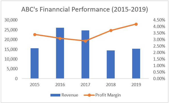
For me, advanced charts are usually. combination charts that allow you to convey a lot more than a regular chart.

For example, a combination chart would be a bar chart that also has a line on a secondary access.

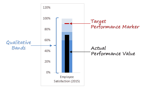
Or a bullet chart or gauge chart (which are not available as built-in chart formats but can be made in Excel).

Another example of an advanced chart would be using interactive controls such as checkboxes or scroll bars to make your chart dynamic.

For example, if you are showing multiple years of data in a bar chart, you can give the option to the user to select the years for which the data should be shown on the chart.

You can click here to read my article on advanced chart types that you can easily create in Excel.

Import Data into Excel

While the analysis can be done in Excel, your data can come from many different sources, such as a database, the web, a text file, an XML file, a CSV file, a DAT file, etc.

While novices would try to copy and paste data into Excel, advanced Excel users would use the built-in data import tools, which are available in the Data tab in the ribbon.

Excel has also released a powerful tool called Power Query that is extremely efficient in connecting to different data sources and fetching that data into Excel.

Power Query

Power Query (also called Get & Transform) is a relatively new feature in Excel that allows you to connect to multiple data sources, transform that data, and then load it into your Excel sheet. All this happens in a separate window called the Power Query Editor.

It’s like having a magical funnel where you pour in raw, messy data and outcomes neatly organized information.

One area where I find Power Query really useful is connecting it to multiple Excel files, then getting all this data and Power Query, then combining this data into one Excel table, and then getting it in an Excel sheet.

Earlier, I had to do this manually, but with Power Query, I can easily combine 2, 5, 10, or even 100 Excel files at once.

Not only this…

Before you get this data in Excel, you can transform the data, such as cleaning the data to remove empty rows or columns or removing duplicates, changing the format of some cells, etc.

Already convinced about the power of Power Query?

No?

Let me explain a scenario that should definitely convert you.

For one of my projects, I get different Excel files from different sales rep that has the sales data. Now, I need to combine all these files to have all the sales data in one single file.

And this needs to be done every week.

So, instead of doing it manually like a caveman, I use Power Query to connect to a folder that has all these files and then combine them,

But wait, here is the best part!

Next week, when I get these new files, I will simply replace the files in the folder and then refresh the query.

That’s it!

I set it once, and then I can reuse it every week (this literally saved me hundreds of hours of work)

Personally, I think Power Query is just as powerful as Pivot Tables, VBA, or Excel formulas.

If you’re new to power query and don’t know where to start, check out my free Power Query video course.

VBA

VBA (Visual Basic for Applications) is a programming language developed by Microsoft for automating tasks in MS Office applications.

In Excel, you can write VBA code to create custom functions, automate repetitive tasks, and even create complex programs like a mini inventory system.

Of all the Excel skills I have covered in this article, VBA is probably the hardest to learn.

While VBA is relatively easier to learn compared to other programming languages, such as Java, it still has a big learning curve for someone who has never learned any programming language.

But if you have already learned any kind of programming language, you can easily get the hang of VBA.

VBA can take your efficiency to a whole new level. You can do things that would otherwise not be possible in Excel. You can automate simple repetitive tasks to complex multistep operations.

One thing that I really like about VBA is that it allows you to create custom functions that can be used as regular worksheet functions. So, if there is something you are not able to achieve using inbuilt Excel functions, you can create a custom function to do it.

If you’re interested in learning VBA, I have a completely free Excel VBA Course that you can check out.

You can also check out all the VBA articles I have on this site on this link.

Other Excel articles you may also like:

• FREE Excel Templates for Your Daily Use
• Free Excel Dashboard Course
• How to Insert Symbols in Excel