

If you want to multiply two columns of numbers together and add up the results in one step, the SUMPRODUCT function is what you’re looking for. It multiplies matching items from each range and then sums those products for you.
That sounds simple, but it’s also the trick that lets SUMPRODUCT count and sum with conditions, handle OR logic, and calculate weighted averages, all from a single formula.
SUMPRODUCT returns one value, but it also works inside dynamic array formulas, so you can feed it a spilled range or a FILTER result.
In this article I’ll show you how to use SUMPRODUCT in Excel, starting with a plain multiply-and-add and building up to conditional counts, conditional sums, OR logic, and the double-unary trick.
SUMPRODUCT Syntax
Here is the syntax of the SUMPRODUCT function:
=SUMPRODUCT(array1, [array2], [array3], ...)
- array1 – the first range (or array) whose values you want to multiply and add.
- [array2], [array3], … – optional extra ranges to multiply against the first, matching item by item. You can pass up to 255 arrays.
With a single array, SUMPRODUCT just adds up its values. With two or more, it multiplies the matching cells first, then sums those products.
Pro Tip: Every array you pass must have the same number of rows and columns. If they don’t line up, SUMPRODUCT returns a #VALUE! error, so keep all your ranges the same size.
SUMPRODUCT works in Excel for Microsoft 365, Excel 2024, 2021, 2019, 2016, and older versions, plus Excel on the web. It never needs Ctrl+Shift+Enter, even in old versions, which is a big part of why people like it.
When to Use SUMPRODUCT
Use the SUMPRODUCT function when you need to:
- Multiply two or more columns row by row and add up the results (like quantity times price).
- Sum or count rows that meet one or more conditions, including OR conditions.
- Calculate a weighted average in a single formula.
- Do array math without pressing Ctrl+Shift+Enter.
Let me show you a few practical examples of how this works.
Example 1: Multiply Two Columns and Sum the Result
Let’s start with the job SUMPRODUCT was built for: multiplying two columns and adding up the answers.
Below is an order table with the product in column A, the quantity ordered in column B, and the unit price in column C. I want the total value of the whole order.
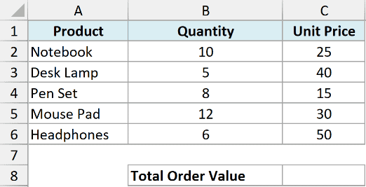
I want to multiply each quantity by its unit price and then add all of those line totals together, without a helper column.
Here is the formula:
=SUMPRODUCT(B2:B6,C2:C6)
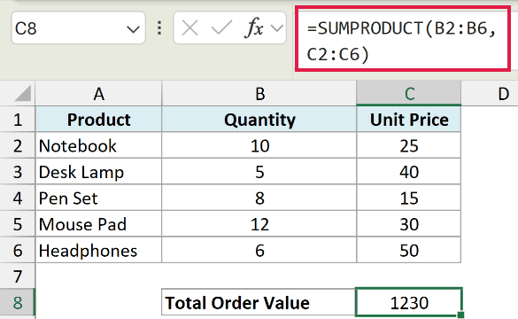
This returns 1230.
SUMPRODUCT walks down both ranges together. It multiplies 10 by 25, 5 by 40, 8 by 15, and so on, giving each row’s line total. Then it adds those five products into one number.
Without SUMPRODUCT you’d add a helper column of quantity times price and then run a SUM on it. SUMPRODUCT folds both steps into one formula.
Example 2: Calculate a Weighted Average
Here’s where SUMPRODUCT really earns its keep. A weighted average gives more pull to the items that matter more, and SUMPRODUCT handles it cleanly.
Below I have a list of products with their average star rating in column B and the number of reviews in column C. I want the overall average rating, weighted by how many reviews each product got.
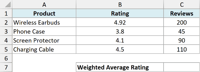
A plain average would treat a product with 200 reviews the same as one with 45. I want the products with more reviews to count more.
Here is the formula:
=SUMPRODUCT(B2:B5,C2:C5)/SUM(C2:C5)
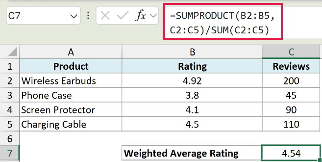
This returns 4.54.
Here is how this formula works:
- SUMPRODUCT(B2:B5,C2:C5) multiplies each rating by its review count and adds the results, giving 2019.
- SUM(C2:C5) adds up all the review counts, giving 445.
- Dividing 2019 by 445 gives the weighted average of 4.54.
A plain =AVERAGE(B2:B5) here would return 4.33, since it ignores the review counts. The weighted version is higher because the top-rated product also has the most reviews.
Example 3: Sum With a Single Condition
SUMPRODUCT can also add up numbers that meet a condition, which is the base trick behind everything that follows.
Below is a sales table with the region in column A, the product in column B, and the sales amount in column C. I want the total sales for the East region only.
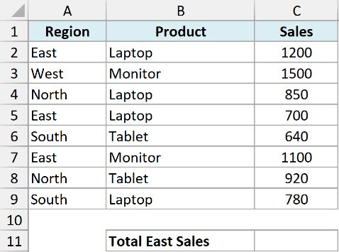
I want to add up column C, but only for the rows where the region in column A is East.
Here is the formula:
=SUMPRODUCT((A2:A9="East")*C2:C9)
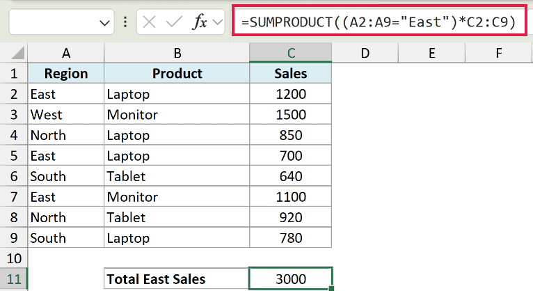
This returns 3000.
The (A2:A9="East") part builds a list of TRUE and FALSE values, one per row. When you multiply that by the sales in column C, TRUE acts as 1 and FALSE acts as 0.
So East rows keep their sales amount and every other row becomes 0. SUMPRODUCT then adds what’s left, which is just the East sales: 1200, 700, and 1100.
Example 4: Count Rows That Meet Two Conditions
Now let’s count instead of sum. This is the classic SUMPRODUCT technique from before COUNTIFS existed, and it still comes in handy.
I’m using the same sales table, with the region in column A and the product in column B. I want to count how many orders were East region AND a Laptop.
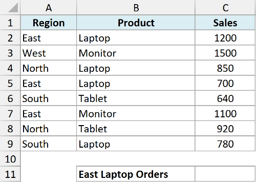
I want the number of rows where two things are both true at once: the region is East and the product is Laptop.
Here is the formula:
=SUMPRODUCT((A2:A9="East")*(B2:B9="Laptop"))
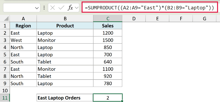
This returns 2.
Each condition makes its own list of TRUE and FALSE values. Multiplying them gives 1 only when both are TRUE in the same row, and 0 otherwise.
So a row counts as 1 only when the region is East and the product is Laptop. SUMPRODUCT adds those 1s up, and two rows match.
Pro Tip: Multiplying conditions together is an AND. Every condition has to be TRUE in a row for that row to count. To combine conditions with OR instead, you add them, which is the next example.
Example 5: Sum With an OR Condition
The multiply pattern handles AND. To handle OR, where a row counts if any one condition is true, you add the conditions instead of multiplying them.
Here’s the same sales table, with the region in column A and sales in column C. I want the total sales for the East region OR the West region.
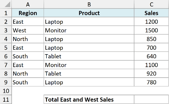
I want to add up sales for any row that is either East or West, and ignore the rest.
Here is the formula:
=SUMPRODUCT(((A2:A9="East")+(A2:A9="West"))*C2:C9)
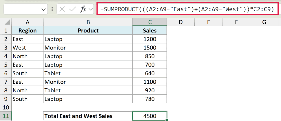
This returns 4500.
Adding the two condition lists gives a 1 for any row that is East or West, and a 0 for the others. Multiplying by the sales column keeps only those rows, and SUMPRODUCT adds them up.
East sales come to 3000 and West sales to 1500, so the total is 4500.
Pro Tip: With OR, make sure a single row can’t satisfy both conditions, or it gets counted twice. Here a region is only ever one value, so that’s not an issue. If two conditions could overlap, that adding trick can double-count.
Example 6: Using the Double Unary (–) to Coerce TRUE and FALSE
When you have just one condition and no other column to multiply by, TRUE and FALSE won’t add up on their own. The double unary (–) converts them into 1s and 0s so SUMPRODUCT can count them.
I’m using the same sales table, with the sales amounts in column C. I want to count how many orders had sales greater than 1000.
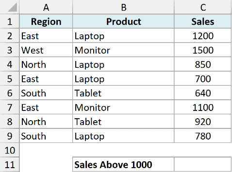
I want a simple count of the rows where the sales value in column C is above 1000.
Here is the formula:
=SUMPRODUCT(--(C2:C9>1000))
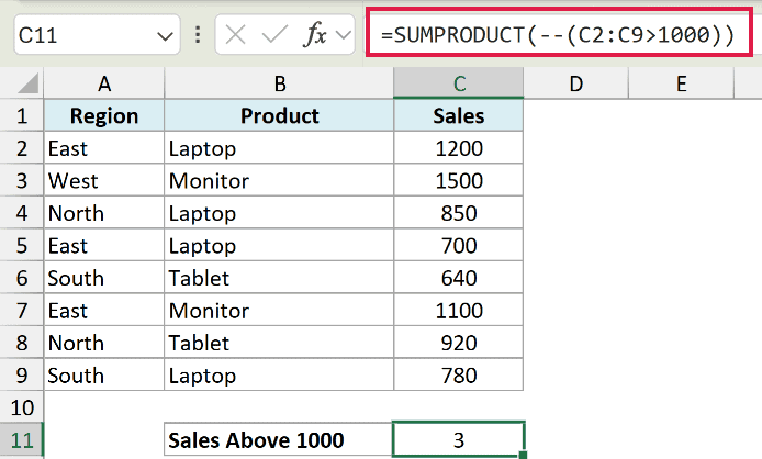
This returns 3.
The (C2:C9>1000) part gives a list of TRUE and FALSE. The two minus signs in front flip each value twice, which turns TRUE into 1 and FALSE into 0 without changing the count.
SUMPRODUCT then adds those 1s and 0s, and three sales figures (1200, 1500, and 1100) clear the 1000 mark.
Pro Tip: You only need the — when a condition stands alone. The moment you multiply it by another array or another condition, that math already turns TRUE and FALSE into 1s and 0s for you.
SUMPRODUCT vs SUMIFS and COUNTIFS
A fair question after all this: why not just use SUMIFS and COUNTIFS? For a lot of the examples above, you could.
The East sales total in Example 3 is also =SUMIF(A2:A9,"East",C2:C9), and the East-Laptop count in Example 4 is also =COUNTIFS(A2:A9,"East",B2:B9,"Laptop"). When a plain SUMIFS or COUNTIFS does the job, reach for it, since it’s easier to read.
SUMPRODUCT still wins in a few spots:
- Math across columns. SUMIFS can’t multiply quantity by price and then sum. SUMPRODUCT does that in one shot (Example 1), and it powers weighted averages (Example 2).
- OR logic in one formula. COUNTIFS only does AND. To count “East or West” you’d add two COUNTIFS, while SUMPRODUCT handles it inline (Example 5).
- Old versions. SUMIFS and COUNTIFS arrived in Excel 2007. On anything older, SUMPRODUCT was the way to do conditional sums and counts.
Tips & Common Mistakes
A few things that trip people up with SUMPRODUCT:
- All arrays must be the same size. If one range has more rows than another, you get a #VALUE! error. Line up every range to the same number of rows and columns.
- Multiply for AND, add for OR. Multiplying condition lists means every condition must be true (AND). Adding them means any one can be true (OR). Mixing them up is the most common SUMPRODUCT bug.
- Use — only for a lone condition. A single condition array needs the double unary (or a
*1) to become numbers. If you’re already multiplying by another array, drop the — because the multiplication coerces the values for you. - Modern SUMIFS and COUNTIFS are often simpler. For a straight conditional sum or count with AND logic, SUMIFS and COUNTIFS read more clearly. Save SUMPRODUCT for column math, OR logic, and weighted averages.
- It plays nicely with dynamic arrays. SUMPRODUCT works on a spilled range too, like
=SUMPRODUCT(FILTER(B2:B6,A2:A6="East"),FILTER(C2:C6,A2:A6="East")), so you can compose it with FILTER and other spill functions.
Wrapping Up
SUMPRODUCT is one of those functions that looks basic and turns out to be a workhorse. Once the multiply-and-add idea clicks, the conditional counts, conditional sums, OR logic, and weighted averages all fall out of the same simple pattern.
Start with a plain two-column multiply, then layer in conditions as you need them. I hope you found this tutorial helpful.
Other Excel Articles You May Also Like:
