Calculating Weighted Average in Excel (Using Formulas)

When we calculate a simple average of a given set of values, the assumption is that all the values carry an equal weight or importance.

For example, if you appear for exams and all the exams carry a similar weight, then the average of your total marks would also be the weighted average of your scores.

However, in real life, this is hardly the case.

Some tasks are always more important than the others. Some exams are more important than the others.

And that’s where Weighted Average comes into the picture.

Here is the textbook definition of Weighted Average:

Now let’s see how to calculate the Weighted Average in Excel.

Calculating Weighted Average in Excel

In this tutorial, you’ll learn how to calculate the weighted average in Excel:

• Using the SUMPRODUCT function.
• Using the SUM function.

So let’s get started.

Calculating Weighted Average in Excel – SUMPRODUCT Function

There could be various scenarios where you need to calculate the weighted average. Below are three different situations where you can use the SUMPRODUCT function to calculate weighted average in Excel

Below are three different situations where you can use the SUMPRODUCT function to calculate weighted average in Excel

Example 1 – When the Weights Add Up to 100%

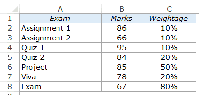
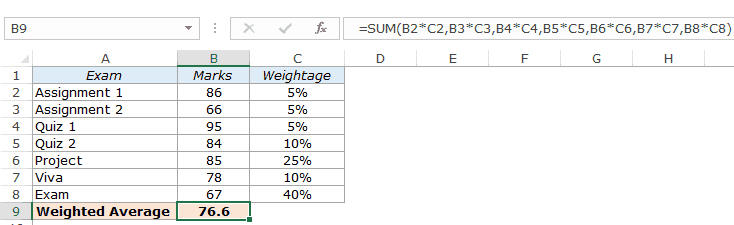
Suppose you have a dataset with marks scored by a student in different exams along with the weights in percentages (as shown below):

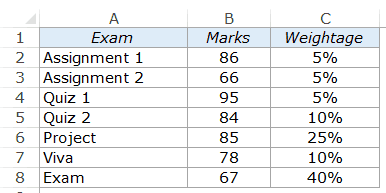
In the above data, a student gets marks in different evaluations, but in the end, needs to be given a final score or grade. A simple average can not be calculated here as the importance of different evaluations vary.

For example, a quiz, with a weight of 10% carries twice the weight as compared with an assignment, but one-fourth the weight as compared with the Exam.

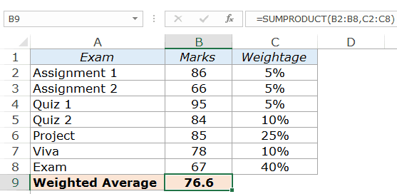
In such a case, you can use the SUMPRODUCT function to get the weighted average of the score.

Here is the formula that will give you the weighted average in Excel:

=SUMPRODUCT(B2:B8,C2:C8)

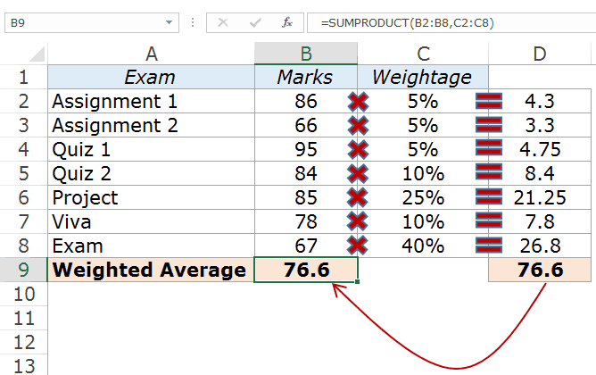
Here is how this formula works: Excel SUMPRODUCT function multiplies the first element of the first array with the first element of the second array. Then it multiplies the second element of the first array with the second element of the second array. And so on..

And finally, it adds all these values.

Here is an illustration to make it clear.

Also read: How to Calculate Percentile in Excel

Example 2 – When Weights Don’t Add Up to 100%

In the above case, the weights were assigned in such a way that the total added up to 100%. But in real life scenarios, it may not always be the case.

Let’s have a look at the same example with different weights.

In the above case, the weights add up to 200%.

If I use the same SUMPRODUCT formula, it will give me the wrong result.

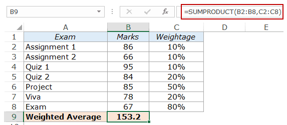
In the above result, I have doubled all the weights, and it returns the weighted average value as 153.2. Now we know a student can’t get more than 100 out of 100, no matter how brilliant he/she is.

The reason for this is that the weights don’t add up to 100%.

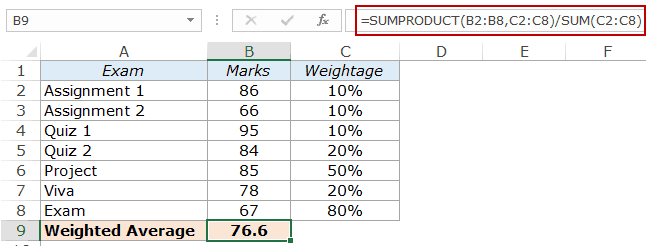
Here is the formula that will get this sorted:

=SUMPRODUCT(B2:B8,C2:C8)/SUM(C2:C8)

In the above formula, the SUMPRODUCT result is divided by the sum of all the weights. Hence, no matter what, the weights would always add up to 100%.

Also read: How to Calculate Percentage Increase in Excel

Example 3 – When the Weights Need to be Calculated

In the example covered so far, the weights were specified. However, there may be cases, where the weights are not directly available, and you need to calculate the weights first and then calculate the weighted average.

Suppose you are selling three different types of products as mentioned below:

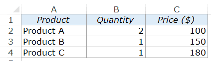
You can calculate the weighted average price per product by using the SUMPRODUCT function. Here is the formula you can use:

=SUMPRODUCT(B2:B4,C2:C4)/SUM(B2:B4)

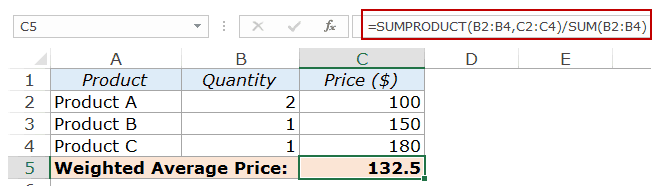
Dividing the SUMPRODUCT result with the SUM of quantities makes sure that the weights (in this case, quantities) add up to 100%.

Also read: How to Calculate Ratios in Excel?

Calculating Weighted Average in Excel – SUM Function

While the SUMPRODUCT function is the best way to calculate the weighted average in Excel, you can also use the SUM function.

To calculate the weighted average using the SUM function, you need to multiply each element, with its assigned importance in percentage.

Using the same dataset:

Here the formula that will give you the right result:

=SUM(B2*C2,B3*C3,B4*C4,B5*C5,B6*C6,B7*C7,B8*C8)

This method is alright to use when you have a couple of items. But when you have many items and weights, this method could be cumbersome and error-prone. There is shorter and better way of doing this using the SUM function.

Continuing with the same data set, here is the short formula that will give you the weighted average using the SUM function:

=SUM(B2:B8*C2:C8)

The trick while using this formula is to use Control + Shift + Enter, instead of just using Enter. Since SUM function can not handle arrays, you need to use Control + Shift + Enter.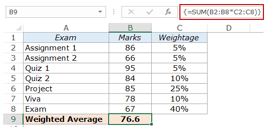

When you hit Control + Shift + Enter, you would see curly brackets appear automatically at the beginning and the end of the formula (see the formula bar in the above image).

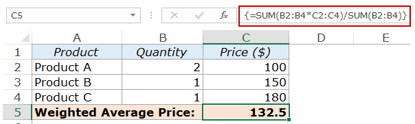
Again, make sure the weights add up to 100%. If it does not, you need to divide the result by the sum of the weights (as shown below, taking the product example):

You May Also Like the Following Excel Tutorials:

• How to Calculate CAGR in Excel
• 5 Easy Ways to Calculate Running Total in Excel (Cumulative Sum)
• How to Calculate IRR in Excel
• Calculating Loan Payment Using PMT Function
• How to Calculate and Format Percentages in Excel
• How to Calculate Age in Excel using Formulas
• Calculating Standard Deviation in Excel
• Calculating Compound Interest in Excel
• Calculating Moving Average in Excel [Simple, Weighted, & Exponential]
• How to Calculate Average Annual Growth Rate (AAGR) in Excel
• Interquartile Range in Excel