
Like many of my Excel tutorials, this one is also inspired by one of the queries I got from a friend. She wanted to calculate the moving average in Excel, and I asked her to search for it online (or watch a YouTube video about it).
But then, I decided to write one myself (the fact that I was somewhat of a statistics nerd in college also played a minor role).
Now, before I tell you how to calculate moving average in Excel, let me quickly give you an overview of what moving average mean and what types of moving averages are there.
In case you want to jump to the part where I show how to calculate moving average in Excel, click here.
Note: I am not an expert on statistics and my intent in this tutorial is not to cover everything about moving averages. I only aim to show you how to calculate moving averages in Excel (with a brief introduction of what moving averages mean).
What is a Moving Average?
I am sure you know what’s an average value.
If I have three days of daily temperature data, you can easily tell me the average of the last three days (hint: you can use the AVERAGE function in Excel to do this).
A Moving Average (also called as the rolling average or running average) is when you keep the time period of the average the same, but keeps moving as new data is added.
For example, on Day 3, if I ask you the 3-day moving average temperature, you will give me the average temperature value of Day 1, 2 and 3. And if on Day 4 I ask you the 3-day moving average temperature, you will give me the average of Day 2, 3, and 4.
As new data is added, you keep the time period (3 days) the same but use the latest data to calculate the moving average.
Moving average is heavily used for technical analysis and a lot of banks and stock-market analysts use it on a daily basis (below is an example I got from the Market Realist site).
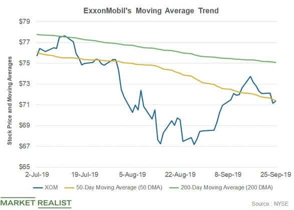
One of the benefits of using the moving averages is that gives you the trend as well as smooths out fluctuations to an extent. For example, in case there is a really hot day, the three-day moving average of the temperature would still make sure that the average value has been smoothened (instead of showing you a really high value that could be an outlier – a one-off instance).
Types of Moving Averages
There are three types of moving averages:
- Simple moving average (SMA)
- Weighted moving average (WMA)
- Exponential moving average (EMA)
Simple Moving Average (SMA)
This is the simple average of the data points in the given duration.
In our daily temperature example, when you simply take an average of the past 10 days, it gives the 10-day simple moving average.
This can be achieved by averaging the data points in the given duration. In Excel, you can do this easily using the AVERAGE function (this is covered later in this tutorial).
Weighted Moving Average (WMA)
Let’s say that the weather is getting cooler with every passing day and you are using a 10-day moving average to get the temperature trend.
Day-10 temperature is more likely to be a better indicator of the trend as compared to Day-1 (since the temperature is dropping with every passing day).
So, we are better off if we rely more on the value of Day 10.
To make this reflect in our moving average, you can give more weight to the latest data and less to past data. This way, you still get the trend, but with more influence of the latest data.
This is called the weighted moving average.
Exponential Moving Average (EMA)
The exponential moving average is a type of weighted moving average where more weight is given to the latest data and it decreases exponentially for the older data points.
It is also called the Exponential Weighted Moving Average (EWMA)
The difference between WMA and EMA is that with WMA, you can assign weights based on any criteria. For example, in a 3-point moving average, you may assign a 60% weight age to the latest data point, 30% to the middle data point and 10% to the oldest data point.
In EMA, a higher weight is given to the latest value and the weight keeps getting exponentially lower for earlier values.
Enough of statistics lecture.
Now let’s dive in and see how to calculate moving averages in Excel.
Also read: How to Find Slope in Excel?
Calculating Simple Moving Average (SMA) using Data Analysis Toolpak in Excel
Microsoft Excel already has an in-built tool to calculate the simple moving averages.
It’s called the Data Analysis Toolpak.
Before you can use the Data Analysis toolpak, you first need to check whether you have it in the Excel ribbon or not. There is a good chance you need to take a few steps to first enable it.
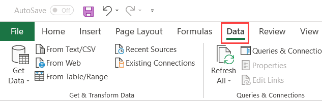
In case you already have the Data Analysis option in the Data tab, skip the steps below and see the steps on calculating moving averages.
Click on the Data tab and check whether you see the Data Analysis option or not. If you don’t see it, follow the below steps to make it available in the ribbon.
- Click the File tab
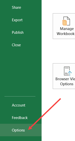
- Click on Options
- In the Excel Options dialog box, click on Add-ins
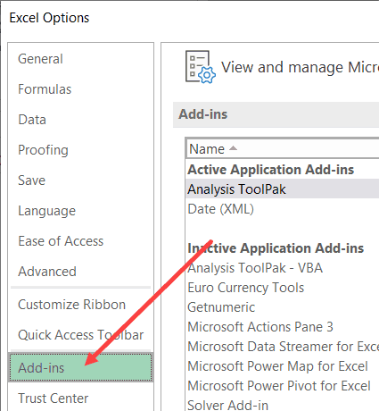
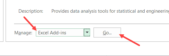
- At the bottom of the dialog box, select Excel Add-ins in the drop-down and then click on Go.
- In the Add-ins dialog box that opens, check the Analysis Toolpak option
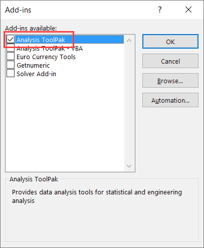
- Click OK.
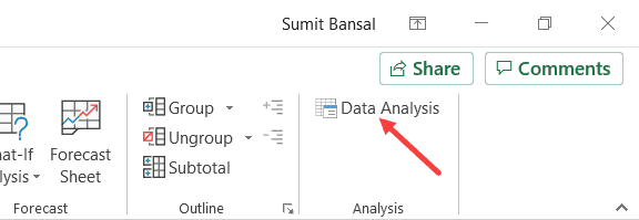
The above steps would enable the Data Analysis Toolpack and you will see this option in the Data tab now.
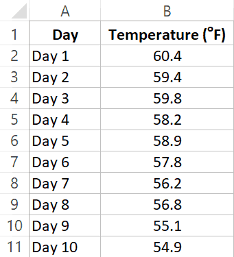
Suppose you have the dataset as shown below and you want to calculate the moving average of the last three intervals.
Below are the steps to use Data Analysis to calculate a simple moving average:
- Click the Data tab
- Click on Data Analysis option
- In the Data Analysis dialog box, click on the Moving Average option (you may have to scroll a bit to reach it).
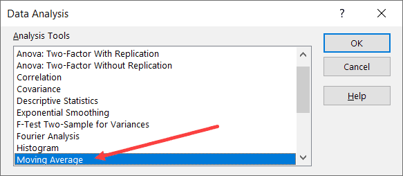
- Click OK. This will open the ‘Moving Average’ dialog box.
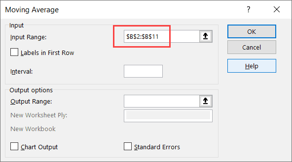
- In the Input Range, select the data for which you want to calculate the moving average (B2:B11 in this example)
- In the Interval option, enter 3 (as we are calculating a three-point moving average)
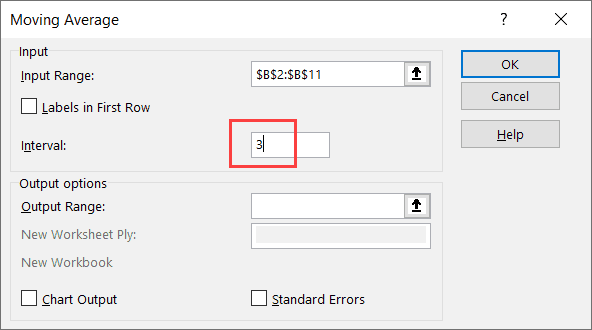
- In the Output range, enter the cell where you want the results. In this example, I am using C2 as the output range
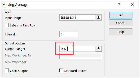
- Click OK
The above steps would give you the moving average result as shown below.
Note that the first two cells in column C have the result as #N/A error. This is because it’s a three-point moving average and needs at least three data points to give the first result. So the actual moving average values start after the third data point onwards.
You will also notice that all this Data Analysis toolpak has done is applied an AVERAGE formula to the cells.
So if you want to do this manually without the Data Analysis toolpack, you can certainly do that.
There are, however, a few things that are easier to do with the data analysis toolpak.
For example, if you want to get the standard error value as well as the chart of the moving average, all you need to do is check a box, and it will be a part of the output.
Also read: Percentage Increase Formula in Excel
Calculating Moving Averages (SMA, WMA, EMA) using Formulas in Excel
You can also calculate the moving averages using the AVERAGE formula.
In fact, if all you need is the moving average value (and not the standard error or chart), using a formula can be a better (and faster) option than using the Data Analysis Toolpak.
Also, Data analysis Toolpak only gives the Simple Moving Average (SMA), but if you want to calculate WMA or EMA, you need to rely on formulas only.
Calculating Simple Moving Average using Formulas
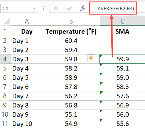
Suppose you have the dataset as shown below and you want to calculate the 3-point SMA:
In the cell C4, enter the following formula:
=AVERAGE(B2:B4)
Copy this formula for all the cells and it will give you the SMA for each day.
Remember: When calculating SMA using formulas, you need to make sure the references on the formula are relative. This means that the formula can be =AVERAGE(B2:B4) or =AVERAGE($B2:$B4), but it can not be =AVERAGE($B$2:$B$4) or =AVERAGE(B$2:B$4). The row number part of the reference needs to be without the dollar sign. You can read more about absolute and relative references here.
Since we are calculating a 3-point Simple Moving Average (SMA), the first two cells (for the first two days) are empty and we start using the formula from the third day onwards. If you want, you can use the first two values as is, and use the SMA value from the third one onwards.
Calculating Weighted Moving Average using Formulas
For WMA, you need to know the weights that would be assigned to the values.
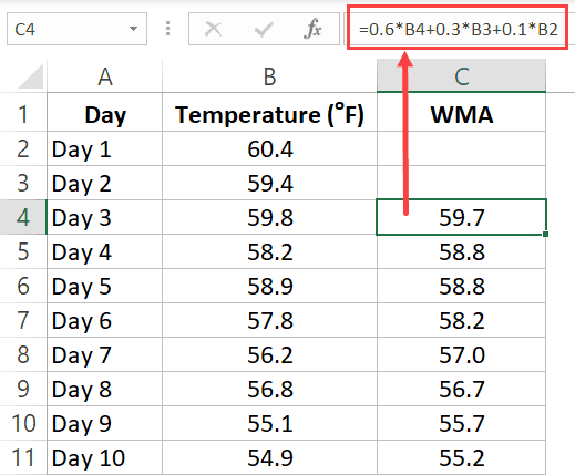
For example, suppose you need to calculate the 3 point WMA for the below dataset, where 60% weight is given to the latest value, 30% to the one before it and 10% of the one before it.
To do this, enter the following formula in cell C4 and copy for all cells.
=0.6*B4+0.3*B3+0.1*B2
Since we are calculating a 3-point Weighted Moving Average (WMA), the first two cells (for the first two days) are empty and we start using the formula from the third day onwards. If you want, you can use the first two values as is, and use the WMA value from the third one onwards.
Calculating Exponential Moving Average using Formulas
Exponential Moving Average (EMA) gives higher weight to the latest value and the weights keep on getting lower exponentially for earlier values.
Below is the formula to calculate the EMA for a three-point moving average:
EMA = [Latest Value - Previous EMA Value] * (2 / N+1) + Previous EMA
…where N would be 3 in this example (as we are calculating a three-point EMA)
Note: For the first EMA value (when you don’t have any previous value to calculate EMA), simply take the value as is and consider it the EMA value. You can then use this value going forward.
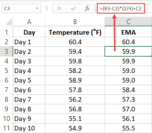
Suppose you have the below data set and you want to calculate the three-period EMA:
In cell C2, enter the same value as in B2. This is because there is no previous value to calculate EMA.
In cell C3, enter the below formula and copy for all cells:
=(B3-C2)*(2/4)+C2
In this example, I have kept it simple and used the latest value and previous EMA value to calculate the current EMA.
Another popular way of doing this is by first calculating the Simple Moving Average and then using it instead of the actual latest value.
Adding Moving Average Trend Line to a Column Chart
If you have a dataset and you’re creating a bar chart using it, you can also add the moving average trend line with a few clicks.
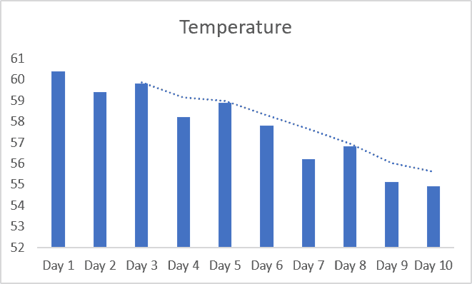
Suppose you have a dataset as shown below:
Below are the steps to create a bar chart using this data and adding a three-part moving average trendline to this chart:
- Select the dataset (including the headers)
- Click the Insert tab
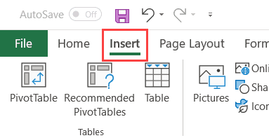
- In the Chart group, click on the ‘Insert Column or Bar chart’ icon.

- Click on the Clustered Column chart option. This will insert the chart in the worksheet.
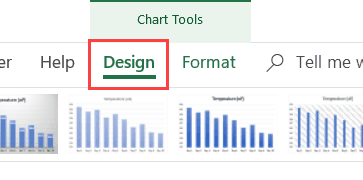
- With the chart selected, click on the Design tab (this tab only appears when the chart is selected)
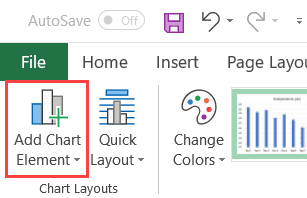
- In the Chart Layouts group, click on ‘Add Chart Element’.
- Hover the cursor on the ‘Trendline’ option and then click on ‘More Trendline Options’
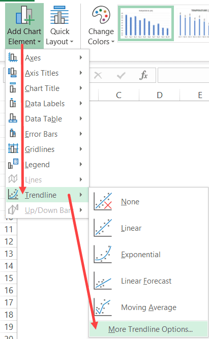
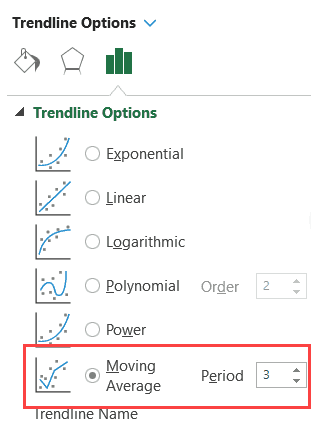
- In the Format Trendline pane, select the ‘Moving Average’ option and set the number of periods.
That’s it! The above steps would add a moving trendline to your column chart.
In case you want to insert more than one moving average trendline (for example one for 2 periods and one for 3 periods), repeat the steps from 5 to 8).
You can use the same steps to insert a moving average trend line to a line chart as well.
Formatting the Moving Average Trend Line
Unlike a regular line chart, a moving average trend line doesn’t allow a lot of formatting. For example, if you want to highlight a specific data point on the trend line, you won’t be able to do that.
A few things you can format in the trendline include:
- Color of the line. You can use this to highlight one of the trendlines by making everything in the chart light in color and making the trendline pop-out with a bright color
- The thickness of the line
- The transparency of the line
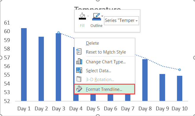
To format the moving average trendline, right-click on it and then select the Format Trendline option.
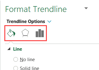
This will open the Format Trendline pane on the right. This pane as all the formatting options (in different sections – Fill & Line, Effects, and Trendline Options).
You may also like the following Excel tutorials:
- What is Standard Deviation and How to Calculate it in Excel?
- How to Calculate Square Root in Excel
- Calculating Weighted Average in Excel
- How to Calculate Compound Annual Growth Rate (CAGR) in Excel
- How to Make a Bell Curve in Excel
- How to Add a TrendLine in Excel Charts
- How to Calculate Average Annual Growth Rate (AAGR) in Excel
- 5 Easy Ways to Calculate Running Total in Excel (Cumulative Sum)
- Calculate MEDIAN IF in Excel
- Weighted Average Calculator
- How to Forecast in Excel (Formulas & Forecast Sheet)


Hi, where you are calculating the 3 day EWMA, why does the formula have n=4?
=(B3-C2)*(2/4)+C2
Is it a typo or a reason it is 4 not 3?
shouldn’t
EMA = [Latest Value – Previous EMA Value] * (2 / N+1) + Previous EMA
be
EMA = [Latest Value – Previous EMA Value] * (2 / (N+1)) + Previous EMA
?
I just scrolled all the way through this blog post, just to tell you THANK YOU!!
I am a suddenly single mom who needs to get back in the workforce after 20+ years as a homeschool mom. Finding your videos has been a blessing from God. You explain everything so clearly. After each concept is taught, I pause the video to try it on my own spreadsheets. I am sharing the link to your videos with all my friends. I hope that this benefits you in someway, as you have benefited me. I could say more wonderful things, but I need to go start lesson 9. 🙂
Thank you so much for the kind words Martha.. I am glad you’re finding the videos useful. More power to you!