How to Calculate Percentage Change in Excel (Increase and Decrease)

If you want to find the percentage increase or decrease between an old and a new number, you can use a simple Excel formula.

Whether you’re working with professional sales data, resource management, project management, or personal data, knowing how to calculate percentage change would help you make better decisions and do better data analysis in Excel.

It’s really easy, thanks to amazing MS Excel features and functions.

In this tutorial, I’ll show you how to calculate percentage change in Excel (i.e., percentage increase or decrease over the given time period), for two values or a whole column.

I’ll also cover month-over-month change and the cases where zero or negative numbers break the usual formula.

So let’s get started!

Percentage Increase Formula for Two Values

The most common scenario is when you have two values and need to find out how much has changed from one value to the other.

For example, if an item’s price increases from $60 to $80, you may want to calculate the percentage increase.

Let’s have a look at examples.

On the “Increase & Decrease” sheet, the Wireless Mouse has an old price of $60 in B2 and a new price of $80 in C2.

The logic is =Change in Price/Original Price. First find the difference between the new and old prices, then divide it by the old price.

Below is the formula to enter in D2:

=(C2-B2)/B2

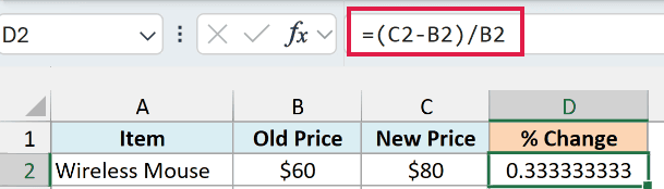
The price has increased by $20. Dividing that change by the original $60 gives 33.33%.

There’s a possibility that you may get the resulting value as a decimal, such as 0.3333. The value is correct, but it needs the right format.

To show this as a percentage value, first select D2, the cell that has the result.

1. Go to the Home tab and click the % button in the Number group.

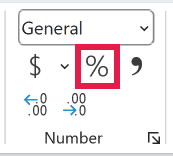
You can also apply the percentage format using the shortcut Ctrl + Shift + %.

2. For more or fewer digits after the decimal, click Increase Decimal or Decrease Decimal, next to the % button in the same group.

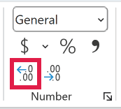
The example file shows two decimal places, so D2 displays 33.33%.

Important: Keep the difference between the new and old price in brackets. This calculates the difference first, then divides it by the original price.

Without brackets, =C2-B2/B2 divides first (following the order of precedence of operators). For the Wireless Mouse, that means 80 – 60/60 = 79, which shows as 7900% with percentage formatting.

As a shorter equivalent, =C2/B2-1 gives the same answer. I use the first formula here because it follows the “change / original” logic directly.

Percentage Decrease Between Two Numbers

Calculating a percentage decrease works the same way as a percentage increase.

On the “Increase & Decrease” sheet, the Desk Lamp has an old price of $80 in B3 and a new price of $60 in C3.

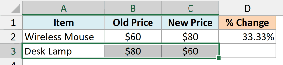
In this case, enter the below formula in D3 to calculate the percentage decrease:

=(C3-B3)/B3

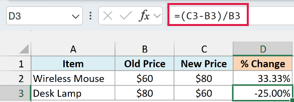
The result is -25.00%. The minus sign tells you it’s a decrease.

We calculate the difference between the new and old price, then divide it by the old price. Here, that’s a $20 drop divided by $80.

Also read: How to Square a Number in Excel

Percent Change for a Whole Column With One Formula

When you have several rows, you can calculate the percent change for the whole column with one formula.

On the “Whole Column” sheet, I have ten grocery items with old prices in B2:B11 and new prices in C2:C11.

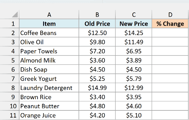
In D2, enter the below formula:

=(C2:C11-B2:B11)/B2:B11

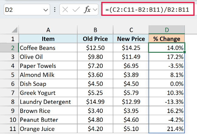
This formula fills D2:D11 on its own. You enter it once, and the results spill into the cells below without dragging or copying.

It subtracts each old price from the matching new price, then divides that difference by the old price in the same row.

For example, Coffee Beans went from $12.50 to $14.25, an increase of 14.0%. Paper Towels went from $7.20 to $6.95, a decrease of 3.5%.

Dish Soap stayed at $4.50, so its result is 0.0%. Format D2:D11 as percentages to show the results this way.

These spill formulas work in Microsoft 365 or Excel 2021 and later. They don’t need Ctrl + Shift + Enter.

For Excel 2019 and earlier, enter the per-row formula below in D2 and copy it down to D11:

=(C2-B2)/B2

Each copied formula calculates the change for its own row.

Month-over-Month Percentage Change

If your numbers are in one column, you can compare each month’s value with the month above it.

On the “Month over Month” sheet, column A has January to December, and B2:B13 has the number of orders for each month.

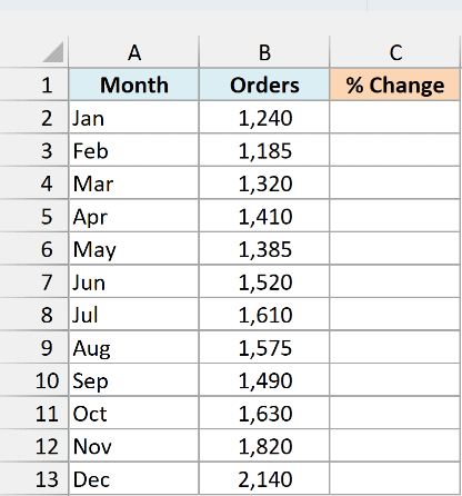
Enter this formula in C3:

=(B3:B13-B2:B12)/B2:B12

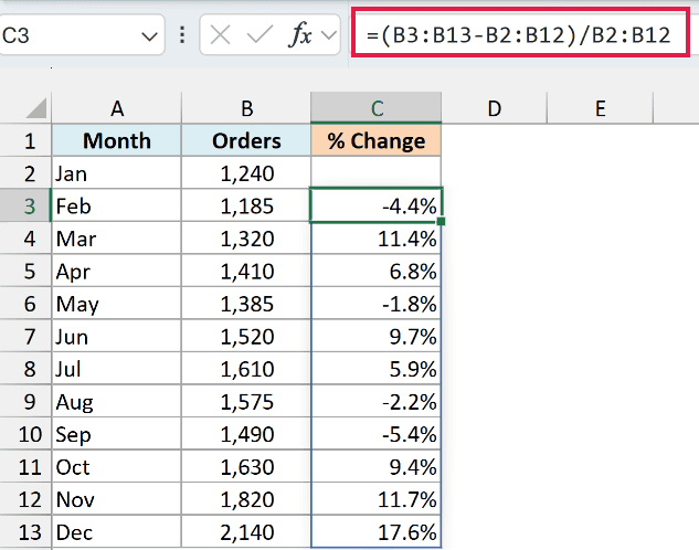
The formula spills down to C13. C2 stays blank because January has no previous month in this dataset to compare with.

B3:B13 is “this month,” starting with February. B2:B12 is the same list shifted up one row, starting with January.

So each month is compared with the one above it. The formula subtracts the previous month’s orders, then divides by that previous month’s value.

January had 1,240 orders and February had 1,185, so February shows -4.4%. March’s 1,320 orders give an 11.4% increase over February.

This also gives you the growth percentage for each month. It compares consecutive months, rather than averaging several months together.

For Excel 2019 and earlier, enter this formula in C3 and copy it down to C13:

=(B3-B2)/B2

For an average growth rate over several periods, see AAGR and CAGR.

Calculate the Value After a Percentage Increase/Decrease

Now let’s look at the other direction. You already know the percentage change and want to calculate the new value.

On the “Value After Change” sheet, I have monthly bills, current costs in B2:B9, and percentage changes in C2:C9.

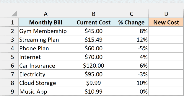
Here, % Change is an input column. You supply the increase or decrease, and the formula calculates the New Cost.

In D2, enter the below formula:

=B2:B9*(1+C2:C9)

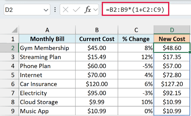
The formula spills down to D9, giving the new cost for all eight bills.

In the above formula, I first add the percentage value to 1 (within brackets).

For the Gym Membership, 1 + 8% is 108%. Multiplying the current $45 cost by 108% gives $48.60.

As you can see, it would work for both percentage increase and percentage decrease.

The Phone Plan has a -5% change, so the formula multiplies $60 by 95% to give $57.00. Electricity drops by 3%, from $95 to $92.15.

For Excel 2019 and earlier, enter this formula in D2, then copy and paste it down to D9:

=B2*(1+C2)

This uses the current cost and percentage change from each row.

Increase/Decrease an Entire Column by a Specific Percentage

You can also apply the same percentage increase or decrease to every value in a column.

On the “Fixed Percentage” sheet, I have eight kitchen appliances with their prices in B2:B9.

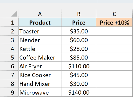
Suppose you want the new prices to be 10% higher. Enter this formula in C2:

=B2:B9*(1+10%)

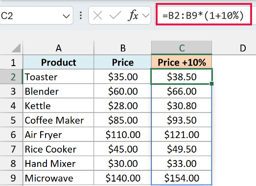
The above formula simply multiplies the old value by 110%, which would end up giving you a value that is 10% higher.

It spills into C2:C9. For the Toaster, the $35 price becomes $38.50.

Similarly, if you want to decrease the entire column by 10%, enter this formula in D2:

=B2:B9*(1-10%)

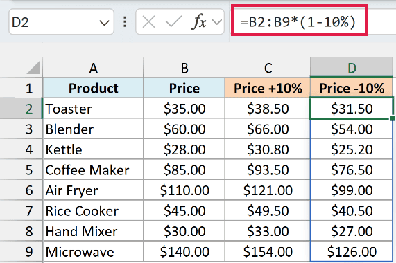
This multiplies each price by 90% and spills down to D9. The Toaster’s price becomes $31.50.

For Excel 2019 and earlier, enter the first formula in C2 and the second in D2 and copy them down to row 9:

=B2*(1+10%)

=B2*(1-10%)

If you have the percentage in a separate cell, you can use the cell reference instead of hardcoding it into the formula.

For the 7% in H1, enter this formula in E2:

=B2:B9*(1+H1)

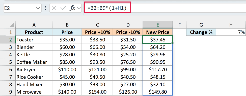
The results spill into E2:E9, with $37.45 for the Toaster.

The benefit of having the percentage change in a separate cell is that you only need to change it in one place. Every formula linked to that cell updates.

The spill formula needs no dollar signs on H1 because you enter it once.

For Excel 2019 and earlier, enter the below per-row formula in E2 and copy it down to E9. Lock H1 as $H$1 so that reference stays fixed:

=B2*(1+$H$1)

For a static approach using Paste Special, see the add or subtract percentage tutorial linked earlier in this article.

Percentage Change With Zero

While calculating percentage change in Excel is quite easy, you will likely face some challenges when there is a zero involved in the calculation.

For example, if your old value is zero and your new value is 100, what do you think is the percentage increase?

On the “Zero Values” sheet, A2:B3 has two examples: an old value of 0 changing to 100, and an old value of 100 changing to 0.

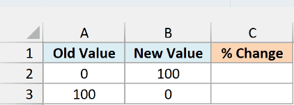
Enter the regular percentage-change formula in C2:

=(B2:B3-A2:A3)/A2:A3

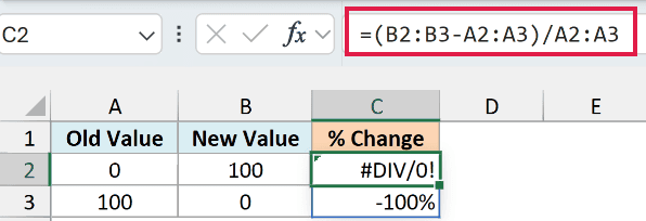
For the first row, the calculation is (100-0)/0. But you can’t divide a number by zero in math, so Excel gives you a division error (#DIV/0!).

This is not an Excel problem, rather it’s a math problem.

Percentage change from zero is undefined. Calling it 100% would make a change from 0 to 5 and a change from 0 to 500 look the same.

A cleaner option is to flag it. Enter this formula in D2:

=IF(A2:A3=0,"N/A",(B2:B3-A2:A3)/A2:A3)

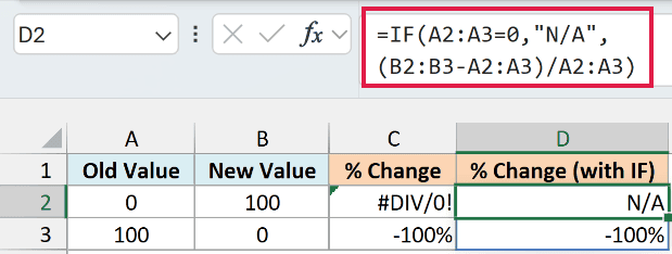
IF checks whether the old value is zero. If it is, the formula returns “N/A”; otherwise, it calculates the percentage change. The results spill into D2:D3.

N/A here is text, so SUM and AVERAGE skip that cell.

IF checks the specific problem we’re trying to handle. IFERROR would also hide unrelated errors, such as text typed into a number cell.

Now, what if you had the opposite.

Suppose your value goes from 100 to 0, as it does in row 3, and you want to calculate the percentage change.

Thankfully, in this case, you can.

The calculation is (0-100)/100, which gives -100%. Both C3 and D3 show this result.

A drop from a positive value to zero is always -100% with the regular formula. From zero, the percentage change is undefined, so flag it instead.

Percentage Change With Negative Numbers

If you have negative numbers involved and you want to calculate the percentage change, things get a bit tricky.

With negative numbers, there could be the following two cases:

1. Both the values are negative.
2. One value is positive and the other is negative. This can mean positive to negative, or negative to positive.

Let’s go through this one by one!

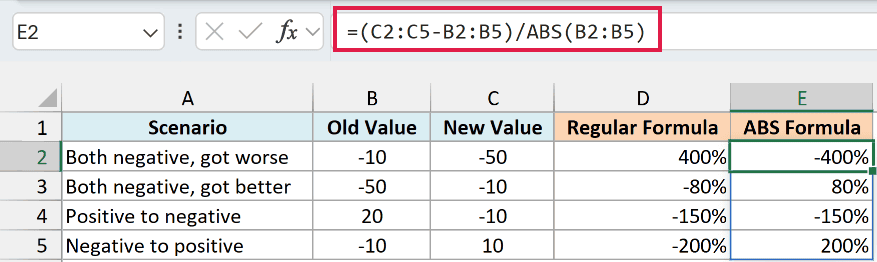
On the “Negative Numbers” sheet, B2:B5 has the old values and C2:C5 has the new values for four scenarios.

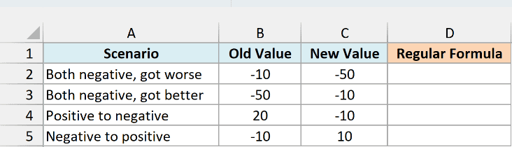
To see what happens with the regular formula, enter this in D2:

=(C2:C5-B2:B5)/B2:B5

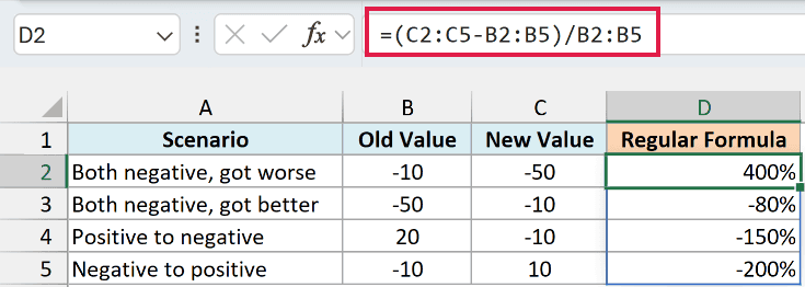
The results spill down to D5. Let’s start with the rows where both values are negative.

In row 2, the value goes from -10 to -50. It got worse, but the regular formula gives a positive 400%.

In row 3, the value improves from -50 to -10, but the formula gives -80%.

The direction is backwards whenever the old value is negative, because dividing by a negative number flips the sign.

Now let’s look at the case where one value is positive and one is negative. There are two possibilities:

1. The old value is positive and the new value is negative.
2. The old value is negative and the new value is positive.

Let’s look at the first scenario!

If the old value is positive, thankfully the math works and you can use the regular percentage formula in Excel.

Row 4 goes from 20 to -10, giving -150%. Since the new value is lower than the old value, the result correctly shows a decline.

So all’s good here!

Now let’s look at the other scenario.

This one needs one minor change.

In row 5, the old value is -10 and the new value is 10. The regular formula gives -200%, which is incorrect as the value change has been positive.

This happens since the denominator in our example is negative. So while the value change is positive, the denominator makes the final result a negative percentage change.

Here is the fix: make the denominator positive.

Enter the below formula in E2 to handle all four cases:

=(C2:C5-B2:B5)/ABS(B2:B5)

The ABS function gives the absolute value, so negative values are automatically changed to positive.

The subtraction stays the same. ABS removes the minus sign from the old value used as the denominator.

The results in E2:E5 are -400%, 80%, -150%, and 200%, matching the direction of each change.

ABS gives the same answer as the regular formula whenever the old value is positive. You can use it for either sign, provided the old value isn’t zero.

ABS gets the direction right, but the size of a change across zero, such as -10 to 10 (200%), is a convention rather than a precise measure, so treat it with care.

For Excel 2019 and earlier, enter this formula in E2 and copy it down to E5:

=(C2-B2)/ABS(B2)

One Formula for Zero and Negative Numbers

If your data has a mixture of positive, zero, and negative values, you can combine the IF check with ABS.

On the “All Cases” sheet, I have eight stores with last year’s profit in B2:B9 and this year’s profit in C2:C9.

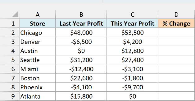
Enter this formula in D2:

=IF(B2:B9=0,"N/A",(C2:C9-B2:B9)/ABS(B2:B9))

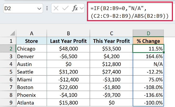
The formula spills into D2:D9. It flags a zero starting value as N/A and otherwise divides the change by the absolute value of last year’s profit.

Here is how it handles three of the stores:

• Austin went from $0 to $12,800. The result is N/A because percentage change from zero is undefined.
• Denver went from -$6,500 to $4,200. The result is 164.6%, showing an improvement from a loss to a profit.
• Phoenix went from -$4,100 to -$9,700. The result is -136.6%, showing that the loss got worse.

For a change from negative to positive, like Denver’s, keep the same convention caveat from the previous section in mind.

For Excel 2019 and earlier, enter this per-row formula in D2 and copy it down to D9:

=IF(B2=0,"N/A",(C2-B2)/ABS(B2))

So these are some methods that you can use to calculate percentage change in Excel, including the cases where an old or new value is zero or negative.

I hope you found this tutorial useful!

Other Excel tutorials you may also like:

• How To Subtract In Excel (Subtract Cells, Column, Dates/Time)
• How to Multiply in Excel Using Paste Special
• How to Stop Excel from Rounding Numbers (Decimals/Fractions)
• How to Add Decimal Places in Excel (Automatically)
• How to Convert Serial Numbers to Dates in Excel
• How to Calculate PERCENTILE in Excel
• Percentage Change Calculator (X% of Y / Increase / Decrease)