Conditional Formatting is one of the most simple yet powerful features in Excel Spreadsheets.
As the name suggests, you can use conditional formatting in Excel when you want to highlight cells that meet a specified condition.
It gives you the ability to quickly add a visual analysis layer over your data set. You can create heat maps, show increasing/decreasing icons, Harvey bubbles, and a lot more using conditional formatting in Excel.
Using Conditional Formatting in Excel (Examples)
In this tutorial, I’ll show you seven amazing examples of using conditional formatting in Excel:
1. Quickly Identify Duplicates
Conditional formatting in Excel can be used to identify duplicates in a dataset.
Here is how you can do this:
- Select the dataset in which you want to highlight duplicates.

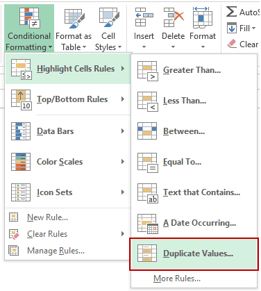
- Go to Home –> Conditional Formatting –> Highlighting Cell Rules –> Duplicate Values.

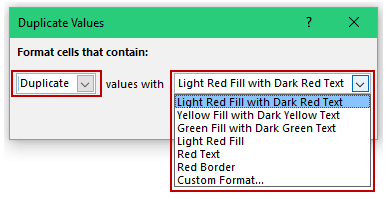
- In the Duplicate Values dialogue box, make sure Duplicate is selected in the left drop down. You can specify the format to be applied by using the right drop down. There are some existing formats that you can use, or specify your own format using the Custom Format option.

- Click OK.

This would instantly highlight all the cells that have a duplicate in the selected data set. Your dataset can be in a single column, multiple columns, or in a non-contiguous range of cells.

See Also: The Ultimate Guide to Find and Remove Duplicates in Excel.
2. Highlight Cells with Value Greater/Less than a Number
You can use conditional formatting in Excel to quickly highlight cells that contain values greater/less than a specified value. For example, highlighting all cells with sales value less than 100 million, or highlighting cells with marks less than the passing threshold.
Here are the steps to do this:
- Select the entire dataset.
- Go to Home –> Conditional Formatting –> Highlighting Cell Rules –> Greater Than.. / Less Than..

- Based on what option you select (greater than or less than), a dialogue box would open. Let’s say, you select the ‘Greater than’ option. In the dialogue box, enter the number in the field on the left. The intent is to highlight cells that have a number greater than this specified number.

- Specify the format to be applied to the cells that meet the condition by using the drop-down on the right. There are some existing formats that you can use, or specify your own format using the Custom Format option.

- Click OK.

This would instantly highlight all the cells with values greater than 5 in a dataset.
The same process can be followed to highlight cells with a value less than a specified values.
Also read: Highlight Cells With Formulas in Excel
3. Highlighting Top/Bottom 10 (or 10%)
Conditional formatting in Excel can quickly identify top 10 items or top 10% from a data set. This could be helpful in situations where you want to quickly see the top candidates by scores or top deal values in the sales data.
Similarly, you can also quickly identify the bottom 10 items or bottom 10% in a dataset.
Here are the steps to do this:
- Select the entire dataset.
- Go to Home –> Conditional Formatting –> Top/Bottom Rules –> Top 10 Items (or %) / Bottom 10 Items (or %).

- Based on what you select, it will open the dialogue box. Let’s say you selected Top 10 items, then it would open a dialogue box as shown below:

- Specify the format to be applied to the cells that meet the condition by using the drop-down on the right. There are some existing formats that you can use, or specify your own format using the Custom Format option.

- Click OK.

This would instantly highlight the top 10 items in the selected dataset. Note that this works only for cells that have a numeric value in it.
Also, if you have less than 10 cells in the dataset, and you select the options to highlight Top 10 items/Bottom 10 Items, then all the cells would get highlighted.
Here are some examples of how the conditional formatting would work:

Also read: Excel Conditional Formatting Based on Another Cell
4. Highlighting Errors/Blanks
If you work with a lot of numerical data and calculations in Excel, you’d know the importance of identifying and treating cells that have errors or are blank. If these cells are used in further calculations, it could lead to erroneous results.
Conditional Formatting in Excel can help you quickly identify and highlight cells that have errors or are blank.
Suppose we have a dataset as shown below:

This data set has a blank cell (A4) and errors (A5 and A6).
Here are steps to highlight the cells that are empty or have errors in it:
- Select the dataset in which you want to highlight blank cells and cells with errors.
- Go to Home –> Conditional Formatting –> New Rule.

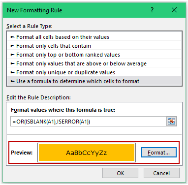
- In the New Formatting Rule dialogue box select Use a formula to determine which cells to format.

- Enter the following formula in the field in the ‘Edit the Rule Description’ section:
=OR(ISBLANK(A1),ISERROR(A1))
- The above formula checks all the cells for two conditions – whether it is blank or not and whether it has an error or not. If any of the conditions is TRUE, it returns TRUE.

- Set the format that you want to apply to the cells that are blank or have errors. To do this, click on the Format button. It will open the ‘Format Cells’ dialogue box, where you can specify the format.

- Click Ok.

This would instantly highlight all the cells that are either blank or have errors in it.

See Also: Using IFERROR and ISERROR to handle errors in excel.
5. Creating Heat Maps
A heat map is a visual representation of data where the color represents the value in a cell. For example, you can create a heat map where a cell with the highest value is colored green and there is a shift towards red color as the value decreases.
Something as shown below:

The above data set has values between 1 and 100. Cells are highlighted based on the value in it. 100 gets the green color, 1 gets the red color.
Here are the steps to create heat maps using conditional formatting in Excel.
- Select the data set.
- Go to Home –> Conditional Formatting –> Color Scales, and choose one of the color schemes.

As soon as you click on the heatmap icon, it would apply the formatting to the dataset. There are multiple color gradients that you can choose from. If you are not satisfied with the existing color options, you can select more rules and specify the color that you want.
Note: In a similar way, you can also apply Data Bard and Icon sets.
6. Highlight Every Other Row/Column
You may want to highlight alternate rows to increase the readability of the data.
These are called the zebra lines and could be especially helpful if you are printing the data.
Now there are two ways to create these zebra lines. The fastest way is to convert your tabular data into an Excel Table. It automatically applied a color to alternate rows. You can read more about it here.
Another way is using conditional formatting.
Suppose you have a dataset as shown below:

Here are the steps to highlight alternate rows using conditional formatting in Excel.
- Select the dataset. In the example above, select A2:C13 (which excludes the header). If you want to include the header as well, then select the entire data set.
- Open the Conditional Formatting dialogue box (Home–> Conditional Formatting–> New Rule) [Keyboard Shortcut – Alt + O + D].

- In the dialogue box, select ‘Use a Formula to determine which cells to format’ dialogue box.

- Enter the following formula in the field in the ‘Edit the Rule Description’ section: =ISODD(ROW())
- The above formula checks all the cells and if the ROW number of a cell is odd, then it returns TRUE. The specified conditional format would be applied to all the cell that return TRUE.

- Set the format that you want to apply to the cells that are blank or have errors. To do this, click on the Format button. It will open the ‘Format Cells’ dialogue box, where you can specify the format.

- Click OK.

That’s it! The alternate rows in the data set will get highlighted.

You can use the same technique in many cases. All you need to do is use the relevant formula in the conditional formatting. Here are some examples:
- Highlight alternate even rows: =ISEVEN(ROW())
- Highlight alternate add rows: =ISODD(ROW())
- Highlight every 3rd row: =MOD(ROW(),3)=0
7. Search and Highlight Data using Conditional Formatting
This one is a bit advanced use of conditional formatting. It would make you look like an Excel rockstar.
Suppose you have a dataset as shown below, with Products Name, Sales Rep, and Geography. The idea is to type a string in cell C2, and if it matches with the data in any cell(s), then that should get highlighted. Something as shown below:

Here are the steps to create this Search and Highlight functionality:
- Select the dataset.
- Go to Home –> Conditional Formatting -> New Rule (Keyboard Shortcut – Alt + O + D).

- In the New Formatting Rule dialogue box, select the option ‘Use a formula to determine which cells to format’.

- Enter the following formula in the field in the ‘Edit the Rule Description’ section: =AND($C$2<>””,$C$2=B5)

- Set the format that you want to apply to the cells that are blank or have errors. To do this, click on the Format button. It will open the ‘Format Cells’ dialogue box, where you can specify the format.

- Click OK.

That’s it! Now when you enter anything in cell C2 and hit enter, it will highlight all the matching cells.
How does this work?
The formula used in conditional formatting evaluates all the cells in the dataset. Let’s say you enter Japan in cell C2. Now Excel would evaluate the formula for each cell.
The formula would return TRUE for a cell when two conditions are met:
- Cell C2 is not empty.
- The content of cell C2 exactly matches the content of the cell in the dataset.
Hence, all the cells that contain the text Japan get highlighted.
Download the Example File

You can use the same logic, to create variations such as:
- Highlight the entire row instead of a cell.
- Highlight even when there is a partial match.
- Highlight the cells/rows as you type (dynamic) [You are going to love this trick :)].
How to Remove Conditional Formatting in Excel
Once applied, conditional formatting remains in place unless you remove it manually. As a best practice, keep the conditional formatting applied only to those cells where you need it.
Since it’s volatile, it may lead to a slow Excel workbook.
To remove conditional formatting:
- Select the cells from which you want to remove conditional formatting.
- Go to Home –> Conditional Formatting –> Clear Rules –> Clear Rules from Selected Cells.
- If you want to remove conditional formatting from the entire worksheet, select Clear Rules from Entire Sheet.

Important things to know about Conditional Formatting in Excel
- Conditional formatting in volatile. It can lead to a slow workbook. Use it only when needed.
- When you copy paste cells that contain conditional formatting, conditional formatting also gets copied.
- If you apply multiple rules on the same set of cells, all rules remain active. In the case of any overlap, the rule applied last is given preference. You can, however, change the order by changing the order from the Manage Rules dialogue box.
You May Also Like the Following Excel Tutorials:


how can i highlight an approaching date i.e. I want a blank cell to change colour as the target date approaches today’s date
Thanks, good content!
Is there a way to make conditional formatting stable when loading data into Excel through PowerQuery?
The issue is that I can add or remove custom columns to loaded data and conditional formatting stays fine, but if I reorder/add/remove columns to source data in PowerQuery, the conditional formatting formulas apply to the unintended column.
In other words, if formula paints red with formula “=AND($P13″China”;$O13″”), applying to “Country” ($P) and “Sales” ($O), when adding/removing/reordering columns in PowerQuery and reload data, coloring applies to i.e. “Product” (now in $P) and “Population” (now in $O), instead of “Country” (now in $Q) and “Sales” now in $B), breaking the whole thing.
I tried =AND(MyTable[Country]”China”;MyTable[Sales]””) but the conditional formatting formula does not seem to accept such a thing as formula-based columns.
Thanks!
learn a lot
I want to protect an excel file with a password which have any type of vba coding
Here there, I need some help with conditional formatting;
what’s the Formula Rule I can use to change color of an entire column if there is less than a specific numbers of charters in that column? For example, I need an eye catcher or attention grabber (change color of column or change to bold) when I have the letter “D” less than 6 or more than 6 times in a column?
Thanks in advance for your help,
Sami
How do I turn a conditionally formatted list into a seperate list that only contains the highlighted cells?
Can anyone help me to solve a small doubt.?
I need cell D5 – D17 to be highlighted in different colors if a specific value comes in the cell F5-F17.
HEY DUDE….IM NOT GETTING SEARCH &HIGHLIGHT DATA USING COND.FORM
Thanks Sumit
Hello – I have comma delimited data (A, A A, B, C, D D, etc) in, say, cells K3 through K99. I want to format another corresponding cell, say H5, or the entire row based on how many such delimited items are in K5. Example, assign red to H5 if K5 has 10 items, assign green if K5 has 5 items, etc. Could anyone help with VB code to do this in excel please?
Is there a way to overlap conditional formatting for a field? Like, if I have a row that displays a color for a range of dates for a project task in a gannt chart, but when I put in a % complete, a range of those rows might highlight over (or replace) the original color indicated by the start and end date.
Love what you did here. I took it one step further and made it toggle Ascending vs. Descending based on what was currently selected. Kind of a hack job in the end, but couldn’t have done it without your help. Thanks!
I want to highlight based on whether a value increased or decreased from the week prior. (less than last week = green, greater than last week = red)
Very good lessons
hii I would like to apply formatting for my task list. the idea is to highlight the cells red with pending task and highlight the cells containing done with green colour. is it possible to do in excel
Yes – You can have a look at the templates I share here. it does exactly what you need. https://trumpexcel.com/excel-to-do-list-template-download/
Hello,
what i’ve done on the search example
AND($C$2″”,ISNUMBER(SEARCH($C$2),B5))
Like this i have a search on partial words.
The examples are very useful. I want to apply conditional formatting to a range depending on a value within that range. I have several range of that type and want to copy paste that condtional formartting to rest all of the individual ranges. Plss plss help me out.
You can copy and paste conditional formatting as well. Just copy the cells which have the conditional formatting and use paste special options to paste format only.
This is really very useful
This is really very useful
Very useful and well explained with examples.
thank u ,really great and simple discussion but what the meaning of Nth Row
Thanks for commenting Mariana.. Nth could be any number. So if you want to highlight every 5th row, you can use the formula =MOD(ROW(),5)=1 in conditional formatting.
Number 6 can be done easier: =isodd(row())
Thanks for sharing.. If one wants to highlight ODD or EVEN rows, then ISODD and ISEVEN functions are better. Else we can you the MOD function
This is really helpful, I really liked this post.
Thanks for commenting Deepak.. Glad you liked it 🙂
Love the 7th one!
Thanks for commenting Greg.. Glad you liked it 🙂
6th is very useful..
Thanks for commenting.. Glad you liked it 🙂
Thank you sir, it is excellent training on excel. Can you send me Gantt chart preparation video.