
Applying conditional formatting in a Pivot Table can be a bit tricky.
Given that Pivot Tables are so dynamic and the data in the backend can change often, you need to know the right way to use conditional formatting in a pivot table in Excel.
The Wrong Way to Apply Conditional Formatting to a Pivot Table
Let’s first look at the regular way of applying conditional formatting in a pivot table.
Suppose you have a pivot table as shown below:
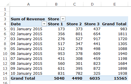
In the above dataset, the date is in the rows and we have store sales data in columns.
Here is the regular way of applying conditional formatting to any dataset:
- Select the data (in this case, we are applying the conditional formatting to B5:D14).
- Go to Home –> Conditional Formatting –> Top/Bottom Rules –> Above Average.

- Specify the format (I am using “Green Fill with Dard Green Text”).

- Click OK.
This will apply the conditional formatting as shown below:
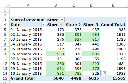
All the data points which are above the average of the entire dataset have been highlighted.
The issue with this method is that it has applied the conditional format to a fixed range of cells (B5:D14). If you add data in the backend and refresh this pivot table, the conditional formatting would not get applied to it.
For example, I go back to the dataset and add data for one more date (11 January 2015). This is what I get when I refresh the Pivot Table.
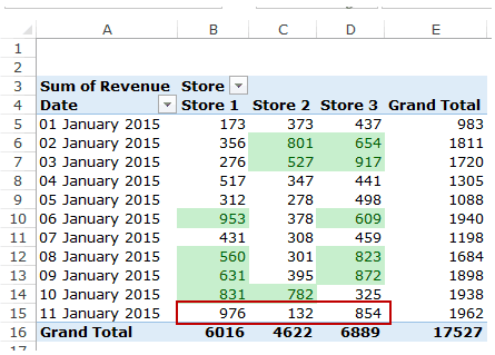
As you can see in the pic above, the data for 11 January 2015 doesn’t get highlighted (while it should as the values for Store 1 and Store 3 are above average).
The reason, as I mentioned above, is that the conditional formatting has been applied on a fixed range (B5:D14), and it doesn’t get extended to new data in the pivot table.
The Right Way to Apply Conditional Formatting to a Pivot Table
Here are two methods to make sure conditional formatting works even when there is new data in the backend.
Method 1 – Using Pivot Table Formatting Icon
This method uses the Pivot Table Formatting Options icon that appears as soon as you apply conditional formatting in a pivot table.
Here are the steps to do this:
- Select the data on which you want to apply conditional formatting.
- Go to Home –> Conditional Formatting –> Top/Bottom Rules –> Above Average.
- Specify the format (I am using “Green Fill with Dard Green Text”).
- Click Ok.
- When you follow the above steps, it applies the conditional formatting on the data set. On the bottom right of the data set, you will see the Formatting Options icon:
- Click on the icon. It will show three options in a drop down:
- Selected Cells (which would be selected by default).
- All cells showing “Sum of Revenue” Values.
- All cells showing “Sum of Revenue” values for “Date” and “Store”.

- Select the third option – All cells showing “Sum of Revenue” values for “Date” and “Store”.

Now when you add any data in the back end and refresh the pivot table, the additional data would automatically be covered by conditional formatting.
Understanding the three options:
- Selected Cells: This is the default option where conditional formatting in applied only on the selected cells.
- All cells showing “Sum of Revenue” Values: In this option, it considers all the cells that show the Sum of Revenue values (or whatever data you have in the values section of the pivot table).
- The issue with this option is that it will also cover the Grand Total values and apply conditional formatting to it.
- All cells showing “Sum of Revenue” values for “Date” and “Store”: This is the best option in this case. It applies the conditional formatting to all the values (excluding Grand Totals) for the combination of Date and Store. Even if you add more data in the back end, this option will take care of it.
Note:
- The Formatting Options icon is visible right after you apply conditional formatting on the data set. If goes away if you do something else (edit a cell or change font/alignment, etc.).
- Conditional formatting goes away if you change the row/column fields. For example, if you remove Date field and apply it again, conditional formatting would be lost.
Method 2 – Using Conditional Formatting Rules Manager
Apart from using the Formatting Options icon, you can also use the Conditional Formatting Rules Manager dialogue box to apply conditional formatting in a pivot table.
This method is useful when you have already applied the conditional formatting and you want to change the rules.
Here is how to do it:
- Select the data on which you want to apply conditional formatting.
- Go to Home –> Conditional Formatting –> Top/Bottom Rules –> Above Average.
- Specify the format (I am using “Green Fill with Dard Green Text”).
- Click Ok. This will apply the conditional formatting to the selected cells.
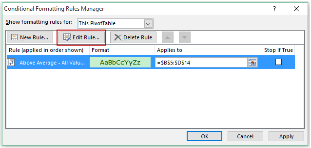
- Go to Home –> Conditional Formatting –> Manage Rules.

- In the Conditional Formatting Rules Manager, select the rule you want to edit and click on Edit Rule button.
- In the Edit Rule dialogue box, you will see the same three options:
- Selected Cells.
- All cells showing “Sum of Revenue” Values.
- All cells showing “Sum of Revenue” values for “Date” and “Store”.

- Select the third option and click OK.
This will apply the conditional formatting to all the cells for ‘Date’ and ‘Store’ fields. Even if you change the backend data (add more store data or date data), the conditional formatting would be functional.
Note: Conditional formatting goes away if you change the row/column fields. For example, if you remove Date field and apply it again, conditional formatting would be lost.
You May Also Like the Following Excel Tutorials:
- Highlight Every Other Row in Excel using Conditional Formatting.
- Creating a Pivot Table in Excel – A Step by Step Tutorial.
- Preparing Source Data For Pivot Table.
- How to Group Numbers in Pivot Table in Excel.
- How to Group Dates in Pivot Tables in Excel.
- How to Refresh Pivot Table in Excel.
- Delete Pivot Table in Excel.
- Using Slicers in Excel Pivot Table.
- How to Add and Use an Excel Pivot Table Calculated Field.
- Pivot Cache in Excel – What Is It and How to Best Use It?
- How to Replace Blank Cells with Zeros in Excel Pivot Tables.


Very useful article. I used Method 2 to fix the conditional formatting that I had already implemented. Thank you!
hi there! Im on a mac and I dont show the same options when I click ‘edit rule’ can you help navigate me on how to get my cond. formatting to stick to my pivots on a mac?
This is helpful
Dear brother Sumit, you are really amazing. You did great job by sharing your knowledge… I strongly believe in sharing knowledge. Sincere appreciation. God bless you dear… I would like to interact with you for Business and personal related requirements, if possible, you may whats up your number on my whats up number 00966535084476. Sanjeeb Rath
Thank You for posting this.
I’m trying to conditional format my shared sites. This reporting is different there are no values meaning counting. We are actually reporting site names. Its hard could you help?
Help! I’m not seeing the icon or the option in ‘Edit Rule’ you are referring to. Is there another route?
I’m in Excel 2013 and I am using “Use a formula to determine which cells to format”, if one of those makes he difference.
Special thanks, same as usual it was wonderful. wish u the best wherever you are .
i would like your help with my data of vehicles that i am having problem with doing pivot line chart
Nice tip. I learned something new today!
Thanks for commenting Mike.. Glad you found this useful 🙂