How to Add and Use an Excel Pivot Table Calculated Field

Often, once you create a Pivot table, there is a need you to expand your analysis and include more data/calculations as a part of it.

If you need a new data point that can be obtained by using existing data points in the Pivot Table, you don’t need to go back and add it in the source data. Instead, you can use a Pivot Table Calculated Field to do this.

Download the dataset and follow along.

What is a Pivot Table Calculated Field?

Let’s start with a basic example of a Pivot Table.

Suppose you have a dataset of retailers and you create a Pivot Table as shown below:

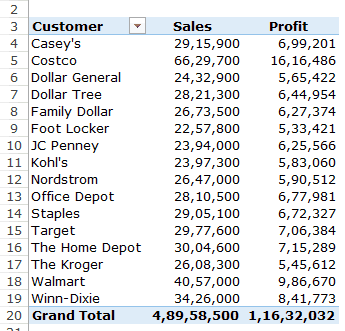
The above Pivot Table summarizes the sales and profit values for the retailers.

Now, what if you also want to know what was the profit margin of these retailers (where the profit margin is ‘Profit’ divided by ‘Sales’).

There are a couple of ways to do this:

1. Go back to the original data set and add this new data point. So you can insert a new column in the source data and calculate the profit margin in it. Once you do this, you need to update the source data of the Pivot Table to get this new column as a part of it.
   • While this method is a possibility, you would need to manually go back to the data set and make the calculations. For example, you may need to add another column to calculate the average sale per unit (Sales/Quantity). Again you will have to add this column to your source data and then update the pivot table.
   • This method also bloats your Pivot Table as you’re adding new data to it.
2. Add calculations outside the Pivot Table. This can be an option if your Pivot Table structure is unlikely to change. But if you change the Pivot table, the calculation may not update accordingly and might give you the wrong results or errors. As shown below, I calculated the Profit Margin when there were retailers in the row. But when I changed it from customers to regions, the formula gave an error.
3. Using a Pivot Table Calculated Field. This is the most efficient way to use existing Pivot Table data and calculate the desired metric. Consider Calculated Field as a virtual column that you have added using the existing columns from the Pivot Table. There are a lot of benefits of using a Pivot Table Calculated Field (as we will see in a minute):
   • It doesn’t require you to handle formulas or update source data.
   • It’s scalable as it will automatically account for any new data that you may add to your Pivot Table. Once you add a Calculate Field, you can use it like any other field in your Pivot Table.
   • It easy to update and manage. For example, if the metrics change or you need to change the calculation, you can easily do that from the Pivot Table itself.

Adding a Calculated Field to the Pivot Table

Let’s see how to add a Pivot Table Calculated Field in an existing Pivot Table.

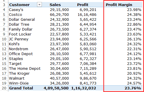
Suppose you have a Pivot Table as shown below and you want to calculate the profit margin for each retailer:

Here are the steps to add a Pivot Table Calculated Field:

• Select any cell in the Pivot Table.
• Go to Pivot Table Tools –> Analyze –> Calculations –> Fields, Items, & Sets.
• From the drop-down, select Calculated Field.
• In the Insert Calculated Filed dialog box:
  • Give it a name by entering it in the Name field.
  • In the Formula field, create the formula you want for the calculated field. Note that you can choose from the field names listed below it. In this case, the formula is ‘= Profit/ Sales’. You can either manually enter the field names or double click on the field name listed in the Fields box.
• Click on Add and close the dialog box.

As soon as you add the Calculated Field, it will appear as one of the fields in PivotTable Fields list.

Now you can use this calculated field as any other Pivot Table field (note that you can not use Pivot Table Calculated Field as a report filter or slicer).

As I mentioned before, the benefit of using a Pivot Table Calculated Field is that you can change the structure of the Pivot Table and it will automatically adjust.

For example, if I drag and drop region in the rows area, you will get the result as shown below, where Profit Margin value is reported for retailers as well as the region.

 In the above example, I have used a simple formula (=Profit/Sales) to insert a calculated field. However, you can also use some advanced formulas.

Before I show you an example of using an advanced formula to create a Pivot Table Calculate Field, here are some things you must know:

• You CAN NOT use references or named ranges while creating a Pivot Table Calculated Field. That would rule out a lot of formulas such as VLOOKUP, INDEX, OFFSET, and so on. However, you can use formulas that can work without references (such SUM, IF, COUNT, and so on..).
• You can use a constant in the formula. For example, if you want to know the forecasted sales where it is forecasted to grow by 10%, you can use the formula =Sales*1.1 (where 1.1 is constant).
• The order of precedence is followed in the formula that makes the calculated field. As a best practice, use parenthesis to make sure you don’t have to remember the order of precedence.

Now, let’s see an example of using an advanced formula to create a Calculated Field.

Suppose you have the dataset as shown below and you need to show the forecasted sales value in the Pivot Table.

For forecasted value, you need to use a 5% sales increase for large retailers (sales above 3 million) and a 10% sales increase for small and medium retailers (sales below 3 million).

Note: The sales numbers here are fake and have been used to illustrate the examples in this tutorial.

Here is how to do this:

•  Select any cell in the Pivot Table.
• Go to Pivot Table Tools –> Analyze –> Calculations –> Fields, Items, & Sets.
• From the drop-down, select Calculated Field.
• In the Insert Calculated Filed dialog box:
  • Give it a name by entering it in the Name field.
  • In the Formula field, use the following formula: =IF(Region =”South”,Sales *1.05,Sales *1.1)
• Click on Add and close the dialog box.

This adds a new column to the pivot table with the sales forecast value.

Click here to Download the dataset.

An Issue With Pivot Table Calculated Fields

Calculated Field is an amazing feature that really enhances the value of your Pivot Table with field calculations, while still keep everything scalable and manageable.

There is, however, an issue with Pivot Table Calculated Fields that you must know before using it.

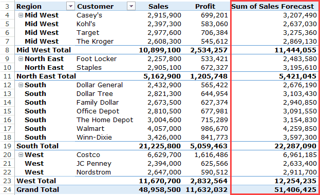
Suppose, I have a Pivot Table as shown below where I used the calculated field to get the forecast sales numbers.

Note that the subtotal and grand totals are not correct.

While these should add the individual sales forecast value for each retailer, in reality, it follows the same calculated field formula that we created.

So for South Total, while the value should be 22,824,000, the South Total wrongly reports it as 22,287,000. This happens as it uses the formula 21,225,800*1.05 to get the value.

Unfortunately, there is no way you can correct this.

The best way to handle this would be to remove subtotals and Grand Totals from your Pivot Table.

You can also go through some innovative workarounds Debra has shown to handle this issue.

How to Modify or Delete a Pivot Table Calculated Field?

Once you have created a Pivot Table Calculated Field, you can modify the formula or delete it using the following steps:

• Select any cell in the Pivot Table.
• Go to Pivot Table Tools –> Analyze –> Calculations –> Fields, Items, & Sets.
• From the drop-down select Calculated Field.
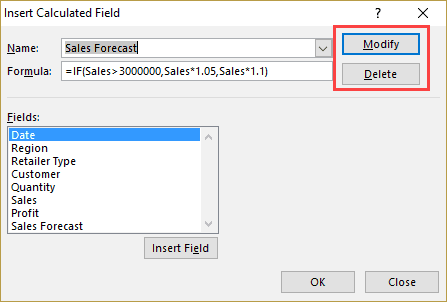
• In the Name field, click on the drop-down arrow (small downward arrow at the end of the field).
• From the list, select the calculated field you want to delete or modify.
• Change the formula in case you want to modify it or click on Delete in case you want to delete it.

How to Get a List of All the Calculated Field Formulas?

If you create a lot of Pivot Table Calculated field, don’t worry about keeping track of the formula used in each one of it.

Excel allows you to quickly create a list of all the formulas used in creating Calculated Fields.

Here are the steps to quickly get the list of All Calculated Fields formulas:

• Select any cell in the Pivot Table.
• Go to Pivot Table Tools –> Analyze –> Fields, Items, & Sets –> List Formulas.

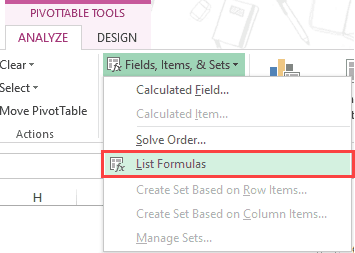
As soon as you click on List Formulas, Excel would automatically insert a new worksheet that will have the details of all the calculated fields/items that you have used in the Pivot Table.

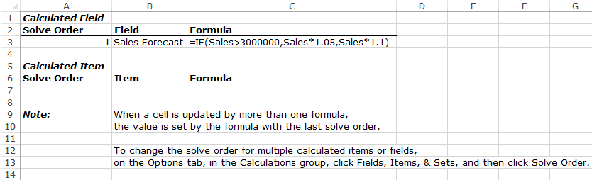
This can be a really useful tool if you have to send your work to the client or share it with your team.

You May Also Find the following Pivot Table Tutorials Useful:

• Preparing Source Data For Pivot Table.
• Using Slicers in Excel Pivot Table: A Beginner’s Guide.
• How to Group Dates in Pivot Tables in Excel.
• How to Group Numbers in Pivot Table in Excel.
• How to Filter Data in a Pivot Table in Excel.
• How to Replace Blank Cells with Zeros in Excel Pivot Tables.
• How to Apply Conditional Formatting in a Pivot Table in Excel.
• Pivot Cache in Excel – What Is It and How to Best Use It?
• How to Delete a Pivot Table in Excel
• How to Show Pivot Table Fields List? (Get Pivot Table Menu Back)