How to Filter Data in a Pivot Table in Excel

There are different ways you can filter data in a Pivot Table in Excel.

As you’ll go through this tutorial, you’ll see there are different data filter options available based on the data type.

Types of Filters in a Pivot Table

Here is a demo of the types of filters available in a Pivot Table.

Let’s look at these filters one by one:

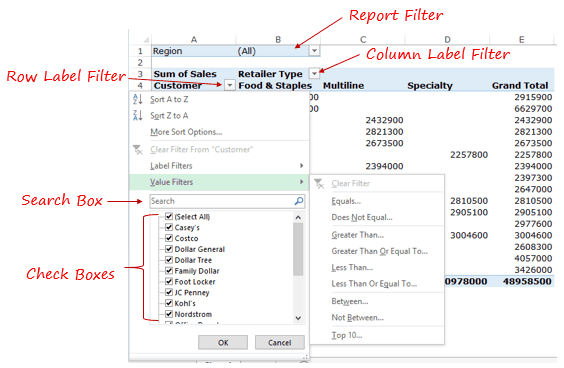
• Report Filter: This filter allows you to drill down into a subset of the overall dataset. For example, if you have retail sales data, you can analyze data for each region by selecting one or more than regions (yes, it allows multiple selections as well). You create this filter by dragging and dropping the Pivot Table field into the Filters area.
• Row/Column Label Filter: These filters allow you to filter relevant data based on the field items (such as filter specific item or item that contains a specific text) or the values (such as filter top 10 items by value or items with a value greater than/less than a specified value).
  • Search Box: You can access this filter within the row/column label filter and this allows you to quickly filter based on the text you enter. For example, if you want data for Costco only, just type Costco here and it will filter that for you.
  • Check Boxes: These allow you to select specific items from a list. For example, if you want to hand pick retailers to analyze, you can do this here. Alternatively, you can also selectively exclude some retailers by unchecking it.

Note, there are two more filtering tools available to a user: Slicers and Timelines (which are not covered in this tutorial).

Let’s see some practical examples of how to use these to filter data in a Pivot Table.

Examples of Using Filters in Pivot Table

The following examples are covered in this section:

• Filter Top 10 Items by Value/Percent/Sum.
• Filter Items based on Value.
• Filter Using Label Filter.
• Filter Using Search Box.

Filter Top 10 Items in a Pivot Table

You can use the top 10 filter option in a Pivot Table to:

• Filter top/bottom items by value.
• Filter top/bottom items that make up a Specified Percent of the Values.
• Filter top/bottom Items that make up a Specified Value.

Suppose you have a Pivot Table as shown below:

Let’s see how to use the Top 10 filter with this data set.

Filter Top/Bottom Items by Value

You can use the Top 10 filter to get a list of top 10 retailers based on the sales value.

Here are the steps to do this:

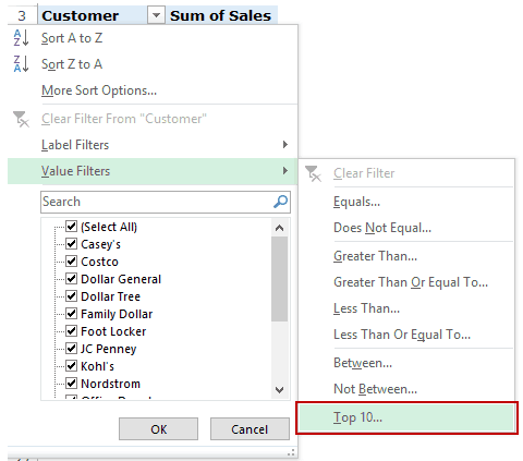
• Go to Row Label filter –> Value Filters –> Top 10.
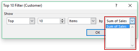
• In the Top 10 Filter dialog box, there are four options that you need to specify:
  • Top/Bottom: In this case since we are looking for top 10 retailers, select Top.
  • The Number of items you want to filter. In this case since we want to get top 10 items, this would be 10.
  • The third field is a drop down with three options: Items, Percent, and Sum. In this case, since we want the top 10 retailers, select Items.
  • The last field lists all the different values listed in the value area. In this case, since we only have the sum of sales, it shows ‘Sum of Sales’ only.

This will give you a filtered list of 10 retailers based on their sales value.

You can use the same process to get the bottom 10 (or any other number) items by value.

Filter Top/Bottom Items that make up a Specified Percent of the Value

You can use the top 10 filter to get a list of top 10 percent (or any other number, say 20 percent, 50 percent, etc.) of items by value.

Let’s say you want to get the list of retailers that make up 25% of the total sales.

Here are the steps to do this:

• Go to Row Label filter –> Value Filters –> Top 10.
• In the Top 10 Filter dialog box, there are four options that you need to specify:
  • Top/Bottom: In this case since we are looking for top retailers that make 25% of the total sales, select Top.
  • In the second field, you need to specify the percent of sales that the top retailers should account for. In this case, since we want to get the top retailers that make 25% of the sales, this would be 25.
  • In the third field, select Percent.
  • The last field lists all the different values listed in the value area. In this case, since we only have the sum of sales, it shows ‘Sum of Sales’ only.

This will give you a filtered list of retailers that make up 25% of the total sales.

You can use the same process to get the retailers that make up the bottom 25% (or any other percentage) of the total sales.

Filter Top/Bottom Items that make up a Specified Value

Let’s say you want to find out the top retailers that account for 20 million in sales.

You can do this using the Top 10 filter in the Pivot Table.

To do this:

• Go to Row Label filter –> Value Filters –> Top 10.
• In the Top 10 Filter dialog box, there are four options that you need to specify:
  • Top/Bottom: In this case since we are looking for top retailers that make 20 million in total sales, select Top.
  • In the second field, you need to specify a value that the top retailers should account for. In this case, since we want to get the top retailers that makeup 20 million in sales, this would be 20000000.
  • In the third field, select Sum. 
  • The last field lists all the different values listed in the value area. In this case, since we only have the sum of sales, it shows ‘Sum of Sales’ only.

This will give you a filtered list of top retailers that make up 20 Million of the total sales.

Filter Items based on Value

You can filter items based on the values in the columns in the values area.

Suppose you have a pivot table created using retail sales data as shown below:

You can filter this list based on the sales value. For example, suppose you want to get a list of all the retailers that have sales more than 3 million.

Here are the steps to do this:

• Go to Row Label filter –> Value Filters –> Greater Than.
• In the Value Filter dialog box:
  • Select the values you want to use for filtering. In this case, it is the Sum of Sales (if you have more items in the values area, the drop down would show all of it).
  • Select the condition. Since we want to get all the retailer with sales more than 3 million, select ‘is greater than’.
  • Enter 3000000 in the last field. 
• Click OK.

This would instantly filter the list and show only those retailers that have sales more than 3 million.

Similarly, there are many other conditions that you can use such as equal to, does not equal to, less than, between, etc.

Filter Data Using Label Filters

Label filters come in handy when you have a huge list and you want to filter specific items based on its name/text.

For example, in the list of retailers, I can quickly filter all the dollar stores by using the condition ‘dollar’ in the name.

Here are the steps to do this:

• Go to Row Label filter –> Label Filters –> Contains.
• In the label filter dialog box:
  • ‘Contains’ is selected by default (since we selected contains in the previous step). You can change this here if you want.
  • Enter the text string for which you want to filter the list. In this case, it is ‘dollar’.
• Click OK.

You can also use wildcard characters along with the text.

Note that these filters are not additive. So if you search for the term ‘Dollar’, it will give you a list of all the stores that have the word ‘dollar’ in it, but if you then again use this filter to get a list using another term, it will filter based on the new term.

Similarly, you can use other label filters such as begins with, ends with does not contain, etc.

Filter Data Using Search Box

Filtering a list using search box is a lot like the contains option in the label filter.

For example, if you have to filter all the retailers that have the name ‘dollar’ in it, simply type dollar in the search box and it will filter the results.

Here are the steps:

• Click on the Label filter drop down and then click on the search box to place the cursor in it.
• Enter the search term, which is ‘dollar’ in this case. You’ll notice that the list gets filtered in the below the search box and you can uncheck any retailer that you want to exclude.
• Click OK.

This would instantly filter all the retailers that contain the term ‘dollar’.

You can use wildcard characters in the search box. For example, if you want to get the name of all the retailers that start with the alphabet T, use the search string as T* (T followed by an asterisk). Since asterisk represents any number of characters, this means that the name can contain any number of characters after T.

Similarly, if you want to get the list of all the retailers that end with the alphabet T, use the search term as *T (asterisk followed by T).

There are a few important things to know about the search bar:

• If you filter once with one criterion and then filter again with another, the first criterion is discarded and you get a list of the second criteria. The filtering is not additive.
• A benefit of using search box is that you can manually deselect some of the results. For example, if you have a huge list of financial companies and you only want to filter banks, you can search for the term ‘bank’. But in case some companies creep in that are not banks, you can simply uncheck it and keep it out.
• You can not exclude specific results. For example, if you want to exclude only the retailers that contain dollar in it, there is no way to do this using the search box. This can, however, be done using the label filter using the ‘does not contain’ condition.

You May Also Like the Following Pivot Table Tutorials:

• Creating a Pivot Table in Excel – A Step by Step Tutorial.
• Preparing Source Data For Pivot Table.
• Group Numbers in Pivot Table in Excel.
• Group Dates in Pivot Tables in Excel.
• Refresh Pivot Table in Excel.
• Delete a Pivot Table in Excel.
• How to Add and Use an Excel Pivot Table Calculated Field.
• Apply Conditional Formatting in a Pivot Table in Excel.
• Pivot Cache in Excel – What Is It and How to Best Use It?
• Replace Blank Cells with Zeros in Excel Pivot Tables.
• Count Distinct Values in Pivot Table