Count Distinct Values in Excel Pivot Table (Easy Step-by-Step Guide)

Excel Pivot Tables are amazing (I know I mention this every time I write about Pivot Tables, but it’s true).

With a basic understanding and a little drag and drop, you can get a bucket-load of work done in a few seconds.

While a lot can be done with a few clicks in Pivot Tables, there are some things that would need a few extra steps or a little bit of work around.

And one such thing is to count distinct values in a Pivot Table.

In this tutorial, I will show you how to count distinct values as well as Unique Values in an Excel Pivot table.

But before I jump into how to count distinct values, it’s important to understand the difference between ‘distinct count’ and ‘unique count’

Distinct Count Vs Unique Count

While these may seem like the same thing, it’s not.

Below is an example where there is a dataset of names and I have listed unique and distinct names separately.

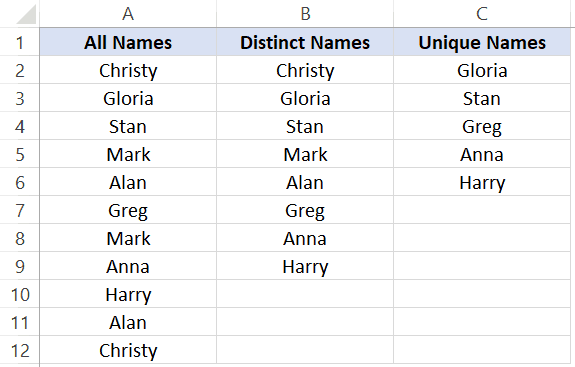
Unique values/names are those that only occur once. This means that all the names that repeat and have duplicates are not unique. Unique names are listed in column C in the above dataset

Distinct values/names are those that occur at least once in the dataset. So if a name appears three times, it’s still counted as one distinct name. This can be achieved by removing the duplicate values/names and keeping all the distinct ones. Distinct names are listed in column B in the above data set.

Count Distinct Values in Excel Pivot Table

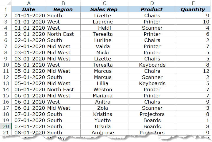
Suppose you have the sales data as shown below:

Click here to download the example file and follow along

With the above dataset, let’s say that you want to find the answer to the following questions:

1. How many sales rep are there in each region (which is nothing but the distinct count of sales reps in each region)?
2. How many sales rep sold the printer in 2020?

While Pivot Tables can instantly summarize the data with a few clicks, to get the count of distinct values, you will need to take a few more steps.

The following two methods are covered in this tutorial:

• Adding a helper column in the original data set to count unique values (works in all versions).
• Adding the data to a data model and using Distinct Count option (available in Excel 2013 and versions after that).

There is a third method which Roger shows in this article (which he calls the Pivot the Pivot Table method).

Let’s get started!

Adding a Helper Column in the Dataset

This is an easy way to count distinct values in the Pivot Table as you only need to add a helper column to the source data. Once you have added a helper column, you can then use this new data set to calculate the distinct count.

While this is an easy workaround, there are some drawbacks to this method (covered later in this tutorial).

Let me first show you how to add a helper column and get a distinct count.

Suppose I have the data set as shown below:

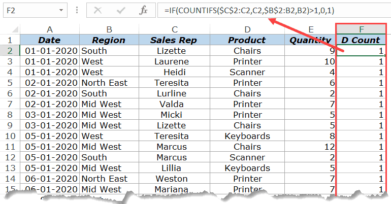
Add the following formula in Column F and apply it for all the cells that have data in the adjacent columns.

=IF(COUNTIFS($C$2:C2,C2,$B$2:B2,B2)>1,0,1)

The above formula uses the COUNTIFS function to count the number of times a name appears in the given region. Also, note that the criteria range is $C$2:C2 and $B$2:B2. This means that it keeps expanding as you go down the column.

For example, in cell E2, the criteria ranges are $C$2:C2 and $B$2:B2 and in cell E3 these ranges expand to $C$2:C3 and $B$2:B3.

This ensures that the COUNTIFS function counts the first instance of a name as 1, the second instance of the name as 2, and so on.

Since we only want to get the distinct names, the IF function is used which returns 1 when a name appears for a region the first time and returns 0 when it appears again. This makes sure that only distinct names are counted and not the repeats.

Below is how your dataset would look like when you have added the helper column.

Now that we have modified the source data, we can use this to create a Pivot Table and use the helper column to get the distinct count of the sales rep in each region.

Below are the steps to do this:

1. Select any cell in the dataset.
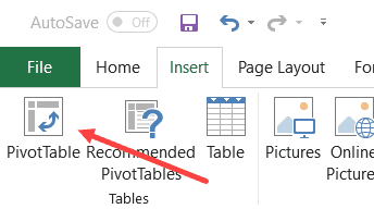
2. Click the Insert Tab.
3. Click on Pivot Table (or use the keyboard shortcut – ALT + N + V)
4. In the Create Pivot Table dialog box, make sure that the Table/Range is correct (and includes the helper column) and’New Worksheet’ in selected.
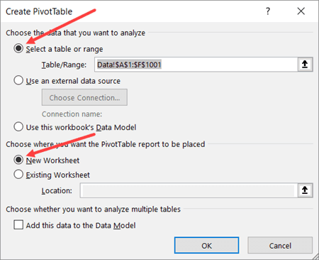
5. Click OK.

The above steps would insert a new sheet which has the Pivot Table.

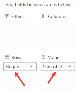
Drag the ‘Region’ field in the Rows area and ‘D Count’ field in the Values area.

You will get a Pivot Table as shown below:

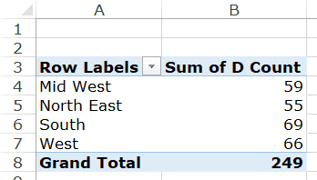
Now you can change the column header from ‘Sum of D count’ to ‘Sales Rep’.

Drawbacks of Using a Helper Column:

While this method is pretty straight forward, I must highlight a few drawbacks that come with modifying the source data in a Pivot Table:

• The data source with the helper column is not as dynamic as a Pivot Table. While you can slice and dice the data any way you want with a Pivot Table, when you use a helper column, you lose a part of that ability. Let’s say that you add a helper column to get the count of a distinct sales rep in each region. Now, what if you also want to get the distinct count of sales rep selling printers. You will have to go back to the source data and modify the helper column formula (or add a new helper column).
• Since you’re adding more data to the Pivot Table source (which also gets added to the Pivot Cache), this can lead to a higher size of Excel file.
• Since we are using an Excel formula, it may make your Excel Workbook slow in case you have thousands of rows of data.

Add Data to Data Model and Summarize Using Distinct Count

Pivot Table added new functionality in Excel 2013 that allows you to get the distinct count while summarizing the data set.

In case you’re using a previous version, you’ll not be able to use this method (as should try adding the helper column as shown in the method above this one).

Suppose you have a dataset as shown below and you want to get the count of the unique sales rep in each region.

Below are the steps to get a distinct count value in the Pivot Table:

1. Select any cell in the dataset.
2. Click the Insert Tab.
3. Click on Pivot Table (or use the keyboard shortcut – ALT + N + V)
4. In the Create Pivot Table dialog box, make sure that the Table/Range is correct and New Worksheet in Selected.
5. Check the box which says – “Add this data to the Data Model”
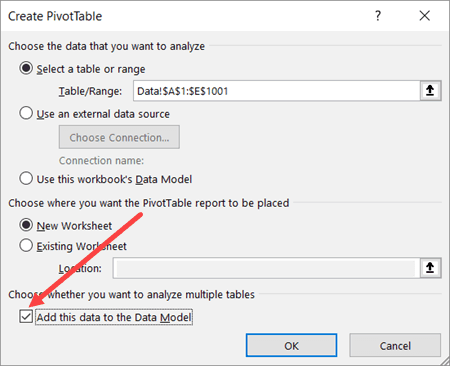
6. Click OK.

The above steps would insert a new sheet which has the new Pivot Table.

Drag the Region in the Rows area and Sales Rep in the Values area. You will get a Pivot Table as shown below:

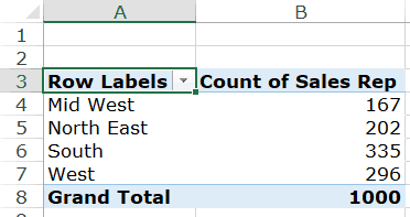
The above Pivot Table gives the total count of the Sales rep in each region (and not the distinct count).

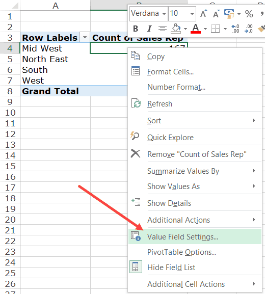
To get the distinct count in the Pivot Table, follow the below steps:

1. Right-click on any cell in the ‘Count of Sales Rep’ column.
2. Click on Value Field Settings
3. In the Value Field Settings dialog box, select ‘Distinct Count’ as the type of calculation (you may have to scroll down the list to find it).
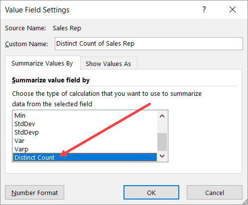
4. Click OK.

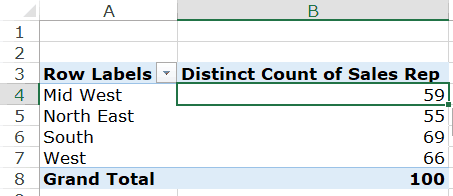
You will notice that the name of the column changes from ‘Count of Sales Rep’ to ‘Distinct Count of Sales Rep’. You can change it to whatever you want.

Some things you know when you add your data to the Data Model:

• If you save your data in the data model and then open in an older version of Excel, it will show you a warning – ‘Some pivot table functions will not be saved’. You may not see the distinct count (and the data model) when opened in an older version that doesn’t support it.
• When you add your data to a Data Model and make a Pivot Table, it will not show the options to add calculated fields and calculated columns.

Click here to download the example file

What If You Want to Count Unique Values (and not distinct values)?

If you want to count unique values, you don’t have any inbuilt functionality in the Pivot Table and will have to rely on helper columns only.

One example could be when you have the below data set and you want to find out how many sales rep are unique to each region. This means that they operate in one specific region only and not the others.

In such cases, you need to create one of more than one helper columns.

For this case, the below formula does the trick:

=IF(IF(COUNTIFS($C$2:$C$1001,C2,$B$2:$B$1001,B2)/COUNTIF($C$2:$C$1001,C2)<1,0,1),IF(COUNTIF($C2:C$22,C2)>1,0,1),0)

The above formula checks whether a sales rep name occurs in one region only or in more than one region. It does that by counting the number of occurrence of a name in a region and dividing it by the total number of occurrences of the name. If the value is less than 1, it indicates that the name occurs in two or more than two regions.

In case the name occurs in more than one region, it returns a 0 else it returns a one.

The formula also checks whether the name is repeated in the same region or not. If the name is repeated, only the first instance of the name returns the value 1, and all other instances return 0.

This may seem a bit complex, but it again depends on what you’re trying to achieve.

So, if you want to count unique values in a Pivot Table, use helper columns and if you want to count distinct values, you can use the inbuilt functionality (in Excel 2013 and above) or can use a helper column.

Click here to download the example file

You May Also Like the Following Pivot Table Tutorials:

• How to Filter Data in a Pivot Table in Excel
• How to Group Dates in Pivot Tables in Excel
• How to Group Numbers in Pivot Table in Excel
• How to Apply Conditional Formatting in a Pivot Table in Excel
• Slicers in Excel Pivot Table
• How to Refresh Pivot Table in Excel
• Delete a Pivot Table in Excel