In this article, I will cover the syntax of COUNTIFS function and how to use in it Excel.
When to use Excel COUNTIFS Function
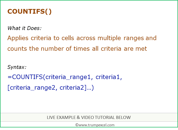
COUNTIFS function can be used when you want to count the number of cells that meet a single or multiple criteria.

What it Returns
It returns a number that represents the number of cells that met a specified criteria in the specified range(s).
Syntax
=COUNTIFS(criteria_range1, criteria1, [criteria_range2, criteria2]…)
Input Arguments
- criteria_range1 – The range of cells for which you want to evaluate against criteria1.
- criteria1 – the criteria which you want to evaluate for criteria_range1 to determine which cells to count.
- [criteria_range2] – The range of cells for which you want to evaluate against criteria2.
- [criteria2] – the criteria which you want to evaluate for criteria_range2 to determine which cells to count.
Additional Notes
- Criteria could be a number, expression, cell reference, text, or a formula.
- Criteria which are text or mathematical/logical symbols (such as =,+,-,/,*) should be in double quotes.
- Wildcard characters can be used in criteria.
- There are three wildcard characters in Excel – the question mark (?), asterisk (*), and tilde (~)
- A question mark matches any single character
- An asterisk matches any sequence of characters.
- If you want to find an actual question mark or asterisk, type a tilde (~) before the character.
- There are three wildcard characters in Excel – the question mark (?), asterisk (*), and tilde (~)
- Criteria are case insensitive (“Hello” and “hello” are treated as same).
- Cells in counted only when all the conditions are met.
- Up to 127 pairs to criteria and criteria range are allowed.
- If the criteria argument is a reference to an empty cell, the COUNTIFS function treats the empty cell as a 0 value
Excel COUNTIFS Function – Live Example
Excel COUNTIFS Function – Video Tutorial
Related Excel Functions:
You May Also Like the Following Tutorials:


