
Excel has many functions where a user needs to specify a single or multiple criteria to get the result. For example, if you want to count cells based on multiple criteria, you can use the COUNTIF or COUNTIFS functions in Excel.
This tutorial covers various ways of using a single or multiple criteria in COUNTIF and COUNTIFS function in Excel.
While I will primarily be focussing on COUNTIF and COUNTIFS functions in this tutorial, all these examples can also be used in other Excel functions that take multiple criteria as inputs (such as SUMIF, SUMIFS, AVERAGEIF, and AVERAGEIFS).
An Introduction to Excel COUNTIF and COUNTIFS Functions
Let’s first get a grip on using COUNTIF and COUNTIFS functions in Excel.
Excel COUNTIF Function (takes Single Criteria)
Excel COUNTIF function is best suited for situations when you want to count cells based on a single criterion. If you want to count based on multiple criteria, use COUNTIFS function.
Syntax
=COUNTIF(range, criteria)
Input Arguments
- range – the range of cells which you want to count.
- criteria – the criteria that must be evaluated against the range of cells for a cell to be counted.
Excel COUNTIFS Function (takes Multiple Criteria)
Excel COUNTIFS function is best suited for situations when you want to count cells based on multiple criteria.
Syntax
=COUNTIFS(criteria_range1, criteria1, [criteria_range2, criteria2]…)
Input Arguments
- criteria_range1 – The range of cells for which you want to evaluate against criteria1.
- criteria1 – the criteria which you want to evaluate for criteria_range1 to determine which cells to count.
- [criteria_range2] – The range of cells for which you want to evaluate against criteria2.
- [criteria2] – the criteria which you want to evaluate for criteria_range2 to determine which cells to count.
Now let’s have a look at some examples of using multiple criteria in COUNTIF functions in Excel.
Using NUMBER Criteria in Excel COUNTIF Functions
#1 Count Cells when Criteria is EQUAL to a Value
To get the count of cells where the criteria argument is equal to a specified value, you can either directly enter the criteria or use the cell reference that contains the criteria.
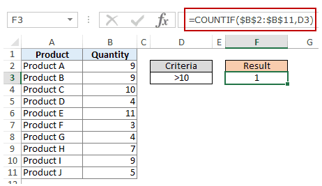
Below is an example where we count the cells that contain the number 9 (which means that the criteria argument is equal to 9). Here is the formula:
=COUNTIF($B$2:$B$11,D3)

In the above example (in the pic), the criteria is in cell D3. You can also enter the criteria directly into the formula. For example, you can also use:
=COUNTIF($B$2:$B$11,9)
#2 Count Cells when Criteria is GREATER THAN a Value
To get the count of cells with a value greater than a specified value, we use the greater than operator (“>”). We could either use it directly in the formula or use a cell reference that has the criteria.
Whenever we use an operator in criteria in Excel, we need to put it within double quotes. For example, if the criteria is greater than 10, then we need to enter “>10” as the criteria (see pic below):
Here is the formula:
=COUNTIF($B$2:$B$11,”>10″)

You can also have the criteria in a cell and use the cell reference as the criteria. In this case, you need NOT put the criteria in double quotes:
=COUNTIF($B$2:$B$11,D3)
There could also be a case when you want the criteria to be in a cell, but don’t want it with the operator. For example, you may want the cell D3 to have the number 10 and not >10.
In that case, you need to create a criteria argument which is a combination of operator and cell reference (see pic below):
=COUNTIF($B$2:$B$11,”>”&D3)
 NOTE: When you combine an operator and a cell reference, the operator is always in double quotes. The operator and cell reference are joined by an ampersand (&).
Also read: Count Cells Less than a Value in Excel (COUNTIF Less Than)
#3 Count Cells when Criteria is LESS THAN a Value
To get the count of cells with a value less than a specified value, we use the less than operator (“<“). We could either use it directly in the formula or use a cell reference that has the criteria.
Whenever we use an operator in criteria in Excel, we need to put it within double quotes. For example, if the criterion is that the number should be less than 5, then we need to enter “<5” as the criteria (see pic below):
=COUNTIF($B$2:$B$11,”<5″)

You can also have the criteria in a cell and use the cell reference as the criteria. In this case, you need NOT put the criteria in double quotes (see pic below):
=COUNTIF($B$2:$B$11,D3)

Also, there could be a case when you want the criteria to be in a cell, but don’t want it with the operator. For example, you may want the cell D3 to have the number 5 and not <5.
In that case, you need to create a criteria argument which is a combination of operator and cell reference:
=COUNTIF($B$2:$B$11,”<“&D3)

NOTE: When you combine an operator and a cell reference, the operator is always in double quotes. The operator and cell reference are joined by an ampersand (&).
#4 Count Cells with Multiple Criteria – Between Two Values
To get a count of values between two values, we need to use multiple criteria in the COUNTIF function.
Here are two methods of doing this:
METHOD 1: Using COUNTIFS function
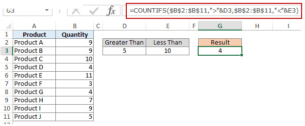
COUNTIFS function can handle multiple criteria as arguments and counts the cells only when all the criteria are TRUE. To count cells with values between two specified values (say 5 and 10), we can use the following COUNTIFS function:
=COUNTIFS($B$2:$B$11,”>5″,$B$2:$B$11,”<10″)

NOTE: The above formula does not count cells that contain 5 or 10. If you want to include these cells, use greater than equal to (>=) and less than equal to (<=) operators. Here is the formula:
=COUNTIFS($B$2:$B$11,”>=5″,$B$2:$B$11,”<=10″)
You can also have these criteria in cells and use the cell reference as the criteria. In this case, you need NOT put the criteria in double quotes (see pic below):

You can also use a combination of cells references and operators (where the operator is entered directly in the formula). When you combine an operator and a cell reference, the operator is always in double quotes. The operator and cell reference are joined by an ampersand (&).
METHOD 2: Using two COUNTIF functions
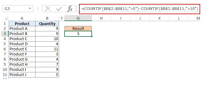
If you have multiple criteria, you can either use COUNTIFS or create a combination of COUNTIF functions. The formula below would also do the same thing:
=COUNTIF($B$2:$B$11,”>5″)-COUNTIF($B$2:$B$11,”>10″)
In the above formula, we first find the number of cells that have a value greater than 5 and we subtract the count of cells with a value greater than 10. This would give us the result as 5 (which is the number of cells that have values more than 5 and less than equal to 10).
If you want the formula to include both 5 and 10, use the following formula instead:
=COUNTIF($B$2:$B$11,”>=5″)-COUNTIF($B$2:$B$11,”>10″)
If you want the formula to exclude both ‘5’ and ’10’ from the counting, use the following formula:
=COUNTIF($B$2:$B$11,”>=5″)-COUNTIF($B$2:$B$11,”>10″)-COUNTIF($B$2:$B$11,10)
You can have these criteria in cells and use the cells references, or you can use a combination of operators and cells references.
Also read: SUM Based on Partial Text Match in Excel (SUMIF)
Using TEXT Criteria in Excel Functions
#1 Count Cells when Criteria is EQUAL to a Specified text
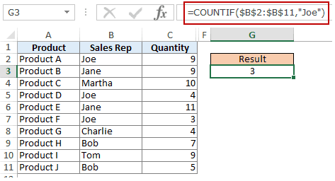
To count cells that contain an exact match of the specified text, we can simply use that text as the criteria. For example, in the dataset (shown below in the pic), if I want to count all the cells with the name Joe in it, I can use the below formula:
=COUNTIF($B$2:$B$11,”Joe”)
Since this is a text string, I need to put the text criteria in double quotes.
You can also have the criteria in a cell and then use that cell reference (as shown below):
=COUNTIF($B$2:$B$11,E3)

NOTE: You can get wrong results if there are leading/trailing spaces in the criteria or criteria range. Make sure you clean the data before using these formulas.
#2 Count Cells when Criteria is NOT EQUAL to a Specified text
Similar to what we saw in the above example, you can also count cells that do not contain a specified text. To do this, we need to use the not equal to operator (<>).
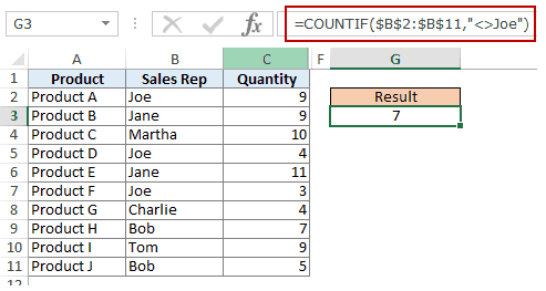
Suppose you want to count all the cells that do not contain the name JOE, here is the formula that will do it:
=COUNTIF($B$2:$B$11,”<>Joe”)
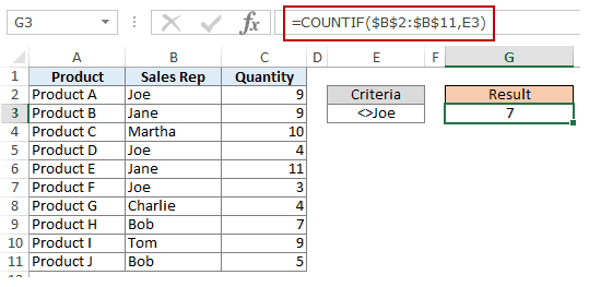
You can also have the criteria in a cell and use the cell reference as the criteria. In this case, you need NOT put the criteria in double quotes (see pic below):
=COUNTIF($B$2:$B$11,E3)
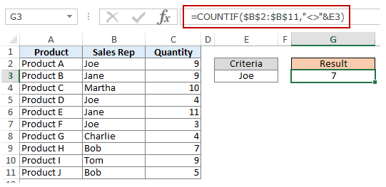
There could also be a case when you want the criteria to be in a cell but don’t want it with the operator. For example, you may want the cell D3 to have the name Joe and not <>Joe.
In that case, you need to create a criteria argument which is a combination of operator and cell reference (see pic below):
=COUNTIF($B$2:$B$11,”<>”&E3)
When you combine an operator and a cell reference, the operator is always in double quotes. The operator and cell reference are joined by an ampersand (&).
Using DATE Criteria in Excel COUNTIF and COUNTIFS Functions
Excel store date and time as numbers. So we can use it the same way we use numbers.
#1 Count Cells when Criteria is EQUAL to a Specified Date
To get the count of cells that contain the specified date, we would use the equal to operator (=) along with the date.
To use the date, I recommend using the DATE function, as it gets rid of any possibility of error in the date value. So, for example, if I want to use the date September 1, 2015, I can use the DATE function as shown below:
=DATE(2015,9,1)
This formula would return the same date despite regional differences. For example, 01-09-2015 would be September 1, 2015 according to the US date syntax and January 09, 2015 according to the UK date syntax. However, this formula would always return September 1, 2105.
Here is the formula to count the number of cells that contain the date 02-09-2015:
=COUNTIF($A$2:$A$11,DATE(2015,9,2))

#2 Count Cells when Criteria is BEFORE or AFTER to a Specified Date
To count cells that contain date before or after a specified date, we can use the less than/greater than operators.
For example, if I want to count all the cells that contain a date that is after September 02, 2015, I can use the formula:
=COUNTIF($A$2:$A$11,”>”&DATE(2015,9,2))

Similarly, you can also count the number of cells before a specified date. If you want to include a date in the counting, use and ‘equal to’ operator along with ‘greater than/less than’ operator.
You can also use a cell reference that contains a date. In this case, you need to combine the operator (within double quotes) with the date using an ampersand (&).
See example below:
=COUNTIF($A$2:$A$11,”>”&F3)

#3 Count Cells with Multiple Criteria – Between Two Dates
To get a count of values between two values, we need to use multiple criteria in the COUNTIF function.
We can do this using two methods – One single COUNTIFS function or two COUNTIF functions.
METHOD 1: Using COUNTIFS function
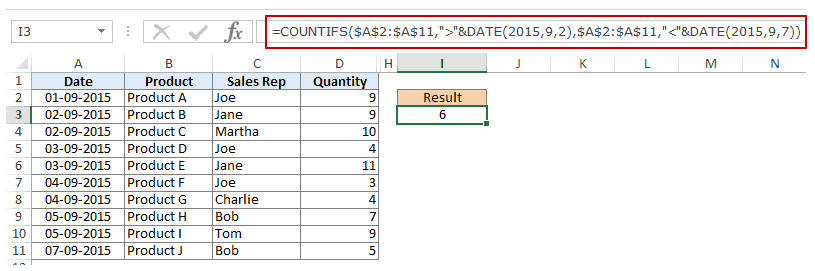
COUNTIFS function can take multiple criteria as the arguments and counts the cells only when all the criteria are TRUE. To count cells with values between two specified dates (say September 2 and September 7), we can use the following COUNTIFS function:
=COUNTIFS($A$2:$A$11,”>”&DATE(2015,9,2),$A$2:$A$11,”<“&DATE(2015,9,7))
The above formula does not count cells that contain the specified dates. If you want to include these dates as well, use greater than equal to (>=) and less than equal to (<=) operators. Here is the formula:
=COUNTIFS($A$2:$A$11,”>=”&DATE(2015,9,2),$A$2:$A$11,”<=”&DATE(2015,9,7))
You can also have the dates in a cell and use the cell reference as the criteria. In this case, you can not have the operator with the date in the cells. You need to manually add operators in the formula (in double quotes) and add cell reference using an ampersand (&). See the pic below:
=COUNTIFS($A$2:$A$11,”>”&F3,$A$2:$A$11,”<“&G3)

METHOD 2: Using COUNTIF functions
If you have multiple criteria, you can either use one COUNTIFS function or create a combination of two COUNTIF functions. The formula below would also do the trick:
=COUNTIF($A$2:$A$11,”>”&DATE(2015,9,2))-COUNTIF($A$2:$A$11,”>”&DATE(2015,9,7))
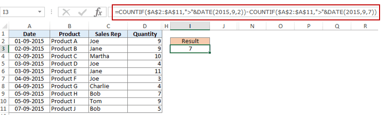
In the above formula, we first find the number of cells that have a date after September 2 and we subtract the count of cells with dates after September 7. This would give us the result as 7 (which is the number of cells that have dates after September 2 and on or before September 7).
If you don’t want the formula to count both September 2 and September 7, use the following formula instead:
=COUNTIF($A$2:$A$11,”>=”&DATE(2015,9,2))-COUNTIF($A$2:$A$11,”>”&DATE(2015,9,7))

If you want to exclude both the dates from counting, use the following formula:
=COUNTIF($A$2:$A$11,”>”&DATE(2015,9,2))-COUNTIF($A$2:$A$11,”>”&DATE(2015,9,7)-COUNTIF($A$2:$A$11,DATE(2015,9,7)))
Also, you can have the criteria dates in cells and use the cells references (along with operators in double quotes joined using ampersand).
Using WILDCARD CHARACTERS in Criteria in COUNTIF & COUNTIFS Functions
There are three wildcard characters in Excel:
- * (asterisk) – It represents any number of characters. For example, ex* could mean excel, excels, example, expert, etc.
- ? (question mark) – It represents one single character. For example, Tr?mp could mean Trump or Tramp.
- ~ (tilde) – It is used to identify a wildcard character (~, *, ?) in the text.
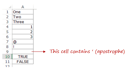
You can use COUNTIF function with wildcard characters to count cells when other inbuilt count function fails. For example, suppose you have a data set as shown below:
Now let’s take various examples:
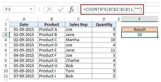
#1 Count Cells that contain Text
To count cells with text in it, we can use the wildcard character * (asterisk). Since asterisk represents any number of characters, it would count all cells that have any text in it. Here is the formula:
=COUNTIFS($C$2:$C$11,”*”)
Note: The formula above ignores cells that contain numbers, blank cells, and logical values, but would count the cells contain an apostrophe (and hence appear blank) or cells that contain empty string (=””) which may have been returned as a part of a formula.
Here is a detailed tutorial on handling cases where there is an empty string or apostrophe.
Here is a detailed tutorial on handling cases where there are empty strings or apostrophes.
Below is a video that explains different scenarios of counting cells with text in it.
#2 Count Non-blank Cells
If you are thinking of using COUNTA function, think again.
Try it and it might fail you. COUNTA will also count a cell that contains an empty string (often returned by formulas as =”” or when people enter only an apostrophe in a cell). Cells that contain empty strings look blank but are not, and thus counted by the COUNTA function.
COUNTA will also count a cell that contains an empty string (often returned by formulas as =”” or when people enter only an apostrophe in a cell). Cells that contain empty strings look blank but are not, and thus counted by the COUNTA function.
So if you use the formula =COUNTA(A1:A11), it returns 11, while it should return 10.
Here is the fix:
=COUNTIF($A$1:$A$11,”?*”)+COUNT($A$1:$A$11)+SUMPRODUCT(–ISLOGICAL($A$1:$A$11))
Let’s understand this formula by breaking it down:
- COUNTIF($N$8:$N$18,”?*”) – This part of the formula returns 5. This includes any cell that has a text character in it. A ? represents one character and * represents any number of characters. Hence, the combination ?* in the criteria forces excel to count cells that have at least one text character in it.

- COUNT($A$1:$A$11) – This counts all the cells that contain numbers. In the above example, it returns 3.

- SUMPRODUCT(–ISLOGICAL($A$1:$A$11) – This counts all the cells that contain logical values. In the above example, it returns 2.

#3 Count Cells that contain specific text
Let’s say we want to count all the cells where the sales rep name begins with J. This can easily be achieved by using a wildcard character in COUNTIF function. Here is the formula:
=COUNTIFS($C$2:$C$11,”J*”)

The criteria J* specifies that the text in a cell should begin with J and can contain any number of characters.
If you want to count cells that contain the alphabet anywhere in the text, flank it with an asterisk on both sides. For example, if you want to count cells that contain the alphabet “a” in it, use *a* as the criteria.
This article is unusually long compared to my other articles. Hope you have enjoyed it. Let me know your thoughts by leaving a comment.
You May Also Find the following Excel tutorials useful:


Can you explain why double quote are needed when using an operator? I use other formulas all the time and put operators without quotes… makes no sense why it is suddenly needed here.
Does anyone know how to write a formula for the following criteria to be met. I can do 2 parts but not combine the formulas as one.
CountIFS ?
Column A = Apple
Column B = Ordered
Coumn C = “in” OR “out” OR “>0”
Any help would be very much appreciated. Thank you.
Hi,
I have to columns that capture the same information (Excellent, Good, Poor, No change), Column M (Performance) and Column N (Performance Update). I want to count pupils performance in such a way that I count Update (N) if both columns have data and the major column (M) if the update is blank. How do i do that?
Is it possible to do COUNTIFS – when cell A “*” and cell L is Blank, must meet 2 conditions. If cell L is not blank then it won’t count.
Thank you,
Hi. Im trying to work out the following criterias to count when these are met.
First i need a range finder:
0-6 less tahn
7-12 greater and less than
13-19 greater and less than
20-26 greater and less than
26+ greater than
Thats two criterias. But i also need it to go to another column to find the sex of the person.
So either a female or a male there
So forexample i need to count the poeple that is greater than/equal to 7 and less than 12 years old while being female or male.
tried for hours now 🙂
Would be great with some help.
=COUNTIFS(‘2019′!B3:B300;”>6″;’2019’!J3:J300;”<=12";'2019'!J3:J300;"Dame")
(I use semicolon isntead of , to break the lines)
0 – 6 : = COUNTIFS(‘Data Source’!$Range1 to look from;”What you are looking for”;’Data Source’!$Range2 for age;”Lower age limit”;’Data Source’!$Range3;”Upper age limit”;’Data Source’!Range4 of City or Country or class;’Filtered Totals Q’!Filtering cell for multiple options for Range4)
fx: =COUNTIFS(‘Data Entry’!$D$3:$D$30002;”Male”;’Data Entry’!$F$3:$F$30002;”>=0″;’Data Entry’!$F$3:$F$30002;”<=6";'Data Entry'!$M$3:$M$30002;'Filtered Totals Q1'!$H$2)
Getting an #VALUE error on: =COUNTIFS($B$16:$D$1000, “Submitted – New”, $E16:$E1000, “Low”)
How to resolve the below issue;
I am trying fill cell AA with 0, if the range C3:C6 is greater than cell J3+2 and cell V3 is greater than 0.
If cell V3=0, I want the cell to fill with “NP”.
I tried using AND and COUNTIF but getting an error. What do I need to change ?
IF(AND(COUNTIF(C3:C6,”>”&(J3+2)),V3>0),0,IF(V3=0, “NP”,1)).
I’m trying to pull back a count of SLAs for a particular month with the count of “Met”. The formula I’m using is:
=COUNTIFS(CONTAIN[Closed Month],Month, CONTAIN[SLA],”*Contain*”,CONTAIN[Contained 4 Hrs], Met)
I have similar formulas in this Dashboard that work fine that are similar, such as:
=COUNTIFS(SLA[Month],Month,SLA[Service Level Description],”*P3*”,SLA[SLA Breach?],FALSE)
Any ideas?
Super
As this is the initial start of my learning Intermediate Excel I would want to learn more on Conditional Formatting with examples and Countif functions in the Indirect Functions as well. I would also want to learn highlighting Datas in Excel using Conditional Formatting.
How can I do countif’s to match multiple columns. Example I have following column header data
Team A Team B League Ground
ABC XYZ Minor Test1
ABC MNO Major Test1
ABC DEF Minor Test1
ABC GEF Minor Test2
I would like count to be
Test1 Test2
Major ABC 1 0
Minor ABC 2 1
Minor XYZ 1 0
Major MNO 1
Minor GEF 0 2
basically I am looking to get count on matching team, league and grounds
TIA
Hi, i am looking for count formula between two hours with in a range(24 hours range is must be unsorted). A2 to A25 given hours as below, now in B2 need answer how many hours count between 8 & 4
anybody can help please?
Time
6
7
8
9
10
11
12
13
14
15
16
17
18
19
20
21
22
23
24
1
2
3
4
5
Hi i have to put formula for multiple range
example: if score 0 to 50% then 1,If 50% to 70% then 2, If 70% to 90% then 3, If 90% and above then 4
I can do with if formula but i want some other option
My friend came to me and gave a task in excel to delete blank row from the data so the worksheet would be convenient to further handling. That sheet has contain more than 20000 thousand rows. So defiantly manually would be like headache!
I did know about ready-made option available to find blank rows but it takes too much processing time and also uses processor.
So I added one column to left most of the data and applied IF and COUNTBLANK formulas …..an i knew the column count is 172.
If I got the 172 in the cell it means the row is blank. And the i attached that cell function to the last row count and Walla…..
I filtered 172 and removed the blank rows and again unfiltered the data….and at the end I have required format of worksheet.
I just took 20 seconds to do that.
You could maybe even just use the sort and filter option and then sorta A-Z so that all of the blank rows come to the top where you can delete them. I’ve done both and find that the sort and filter option is very quick. I’ve used it on data sets with 27,000 rows plus of data. Just thought I’d throw that out there.
Hi,
I’m trying to add days to a date by criteria. For instance:
AE + 21 days
UG + 14 days
Cell B2 “AE or UG” (AE or UG will be inputted by user)
Cell C2 “Date” Known Date such as today’s date 12/22/15
Cell C3 “Date with added days (21 or 14)”
Thanks,
AG
Hello Alex.. What do you mean by AE + 21 or UG + 21. Do you wish to add 14/21 days to the date in cell C2 based on what a user would enter in cell B2. Try this formula: =C2+IF($B$2=”AE”,21,14)
Would be better if you explain this a bit more or share an example file.
Sumit, thank you for replying. AE and UG is a place holder (Name). If the user selects the name AE it will add 21 days to the date from cell B2. If the user selects UG it will add 14 days to the date from cell B2.
The formula you sent works GREAT but how would I add UG and 14 days?
Thank you
For counting non-blank cell, we may use
=COUNTA(Range)-COUNTBLANK(Range)
Interestingly, COUNTBLANK counts blank cells and blank cells returned by formula, as well as a single apostrophe.
Cheers,
wmfexcel.com
EDIT:
the follow should be
=COUNTIF(Range,””””)-COUNTBLANK(Range)
:p
Hey MF.. Thanks for sharing.. we can also get rid of the additional “”. So this also works:
=COUNTIF(Range,””)-COUNTBLANK(Range)