How to Sum a Column in Excel (5 Really Easy Ways)

To get the sum of an entire column is something most of us have to do quite often. For example, if you have the sales data to date, you may want to quickly know the total sum in the column to the sales value till the present day.

You may want to quickly see what the total sum is or you may want is as a formula in a separate cell.

This Excel tutorial will cover a couple of quick and fast methods to sum a column in Excel.

Select and Get the SUM of the Column in Status Bar

Excel has a status bar (at the bottom right of the Excel screen) which displays some useful statistics about the selected data, such as Average, Count, and SUM.

Suppose you have a dataset as shown below and you want to quickly know the sum of the sales for the given weeks.

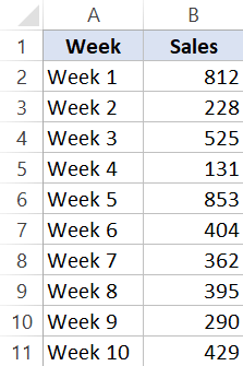
To do this, select the entire Column B (you can do that by clicking on the B alphabet at the top of the column).

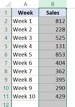
As soon as you select the entire column, you will notice that the status bar shows you the SUM of the column.

This is a really quick and easy way to get the sum of an entire column.

The good thing about using the status bar to get the sum of the column is that it ignores the cells that have the text and only considers the numbers. In our example, cell B1 has the text title, which is ignored and the sum of the column is displayed in the status bar.

In case you want to get the sum of multiple columns, you can make the selection, and it will show you the total sum value of all the selected columns.

In case you don’t want to select the entire column, you can make a range selection, and the status bar will show the sum of the selected cells only.

If you want, you can customize the status bar and get more data such as the maximum or the minimum value from the selection. To do this, right-click on the status bar and make the customizations.

Get the SUM of a Column with AutoSum (with a Single-click/Shortcut)

Autosum is a really awesome tool that allows you to quickly get the sum of an entire column with a single click.

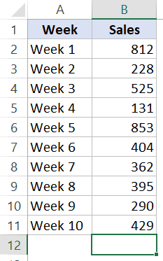
Suppose you have the dataset as shown below and you want to get the sum of the values in column B.

Below are the steps to get the sum of the column:

1. Select the cell right below the last cell in the column for which you want the sum
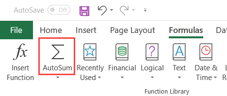
2. Click the Formula tab
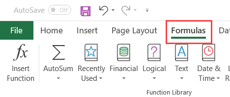
3. In the Function Library group, click on the Autosum option

The above steps would instantly give you the sum of the entire column in the selected cell.

You can also use the Auto-sum by selecting the column that has the value and hitting the auto-sum option in the formula tab. As soon as you do this, it will give you the auto-sum in the cell below the selection.

Note: Autosum automatically detects the range and includes all the cells in the SUM formula. If you select the cell which has the sum and look at the formula in it, you will notice that it refers to all the cells above it in the column.

One minor irritant when using Autosum is that it would not identify the correct range in case there are any empty cells in the range or any cell has the text value. In the case of the empty cell (or text value), the auto-sum range would start below this cell.

AutoSum Keyboard Shortcut

While using the Autosum option in the Formula tab is fast enough, you can make getting the SUM even faster with a keyboard shortcut.

To use the shortcut, select the cell where you want the sum of the column and use the below shortcut:

ALT = (hold the ALT key and press the equal to key)

Using the SUM Function to Manually calculate the Sum

While the auto-sum option is fast and effective, in some cases, you may want to calculate the sum of columns (or rows) manually.

One reason for doing this could be when you don’t want the sum of the entire column, but only of some of the cells in the column.

In such a case, you can use the SUM function and manually specify the range for which you want the sum.

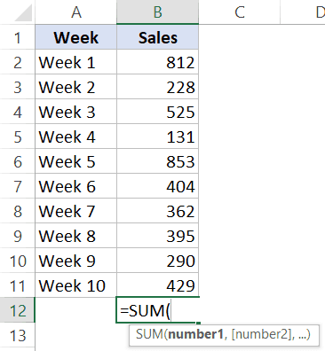
Suppose you have a dataset as shown below and you want the sum of the values in column B:

Below are the steps to use the SUM function manually:

1. Select the cell where you want to get the sum of the cells/range
2. Enter the following: =SUM(
3. Select the cells that you want to sum. You can use the mouse or can use the arrow key (with arrow keys, hold the shift key and then use the arrow keys to select range of cells).
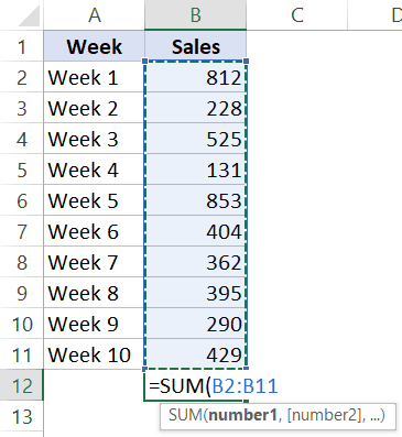
4. Hit the Enter key.

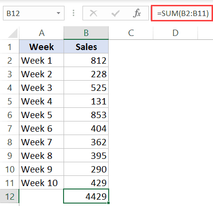
The above steps would give you the sum of the selected cells in the column.

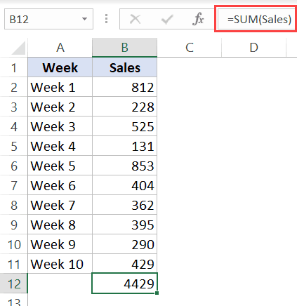
You can also create and use named ranges in the SUM function to quickly get the sum value. This could be useful when you have data spread on a large spreadsheet and you want to quickly get the sum of a column or range. You would first need to create a named range and then you can use that range name to get the sum.

Below is an example where I have named the range – Sales. The below formula also gives me the sum of the sales column:

=SUM(Sales)

Note that when you use the SUM function to get the sum of a column, it will also include the filtered or hidden cells.

In case you want the hidden cells to not be included when summing a column, you need to use the SUBTOTAL or AGGREGATE function (covered later in this tutorial).

Also read:  How to Sum Across Multiple Sheets in Excel?

Sum Only the Visible Cells in a Column

In case you have a dataset where you have filtered cells or hidden cells, you can not use the SUM function.

Below is an example of what can go wrong:

In the above example, when I sum the visible cells, it gives me the result as 2549, while the actual result of the sum of visible cells would be 2190.

The reason we get the wrong result is that the SUM function also takes the filtered/hidden cells when calculating the sum of a column.

In case you only want to get the sum of visible cells, you can’t use the SUM function. In this case, you need to use the AGGREGATE or SUBTOTAL function.

Below is the formula you can use to get the sum of only the visible cells in a column:

=AGGREGATE(9,3,B2:B6)

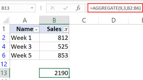
The Aggregate function takes the following arguments:

• function_num: This is a number that tells the AGGREGATE function the calculation that needs to be done. In this example, I have used 9 as I want the sum.
• options: In this argument, you can specify what you want to ignore when doing the calculation. In this example, I have used 3, which ‘Ignores hidden row, error values, nested SUBTOTAL, and AGGREGATE functions’. In short, it only uses the visible cells for the calculation.
• array: This is the range of cells for which you want to get the value. In our example, this is B2:B6 (which also has some hidden/filtered rows)

In case you’re using Excel 2007 or prior versions, you can use the following Excel formula:

=SUBTOTAL(9,B2:B6)

Below is a formula where I show how to sum a column when there are filtered cells (using the SUBTOTAL function)

Convert Tabular Data to Excel Table to Get the Sum of Column

When you convert tabular data to an Excel Table, it becomes really easy to get the sum of columns.

I always recommend converting data into an Excel table, as it offers a lot of benefits. And with new tools such as Power Query, Power Pivot, and Power BI working so well with tables, it’s one more reason to use it.

To convert your data into an Excel table, follow the below steps:

1. Select the data that you want to convert to an Excel Table
2. Click the Insert tab
3. Click on the Table icon
4. In the Create Table dialog box, make sure the range is correct. Also, check the option ‘My table has headers’ in case you have headers in your data.
5. Click Ok.

The above steps would convert your tabular data into an Excel Table.

Once you have the table in place, you can easily get the sum of all the columns.

Below are the steps to get the sum of the columns in an Excel Table:

1. Select any cell in the Excel table
2. Click the Design tab. This is a contextual tab that only appears when you select a cell in the Excel table.
3. In the ‘Table Style Options’ group, check the ‘Total Row’ option

The above steps would instantly add a totals row at the bottom of the table and give the sum of all the columns.

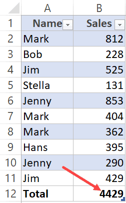
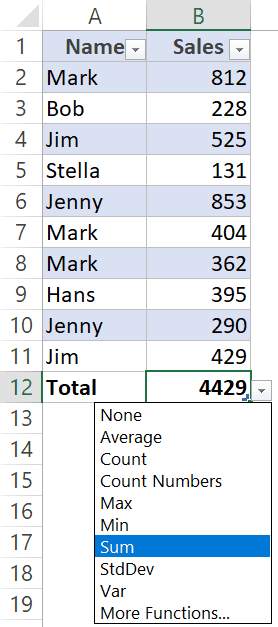
Another thing to know about using an Excel table is that you can easily change the value from the SUM of the column to Average, Count, Min/Max, etc.

To do this, select a cell in the totals rows and use the drop-down menu to select the value you want.

Get the Sum of Column Based on a Criteria

All the methods covered above would give you the sum of the entire column.

In case you want to only get the sum of those values that satisfy a criterion, you can easily do that with a SUMIF or SUMIFS formula.

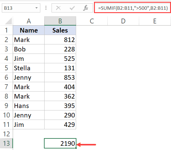
For example, suppose you have the dataset as shown below and you only want to get the sum of those values that are more than 500.

You can easily do this using the below formula:

=SUMIF(B2:B11,">500",B2:B11)

With the SUMIF formula, you can use a numeric condition as well as a text condition.

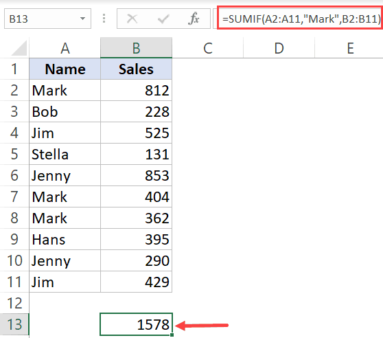
For example, suppose you have a dataset as shown below and you want to get the SUM of all the sales done by Mark.

In this case, you can use column A as the criteria range and “Mark” as the criteria, and the formula will give you the sum of all the values for Mark.

The below formula will give you the result:

=SUMIF(A2:A11,"Mark",B2:B10)

You may also like the following Excel tutorials:

• How to Sum Positive or Negative Numbers in Excel
• How to Apply Formula to the Entire Column in Excel
• How to Compare Two Columns in Excel (for matches and differences)
• How to Unhide COLUMNS in Excel
• How to Count Colored Cells In Excel
• How to Use Multiple Criteria in Excel COUNTIF and COUNTIFS Function
• 100+ Excel Functions (explained with examples)
• 5 Easy Ways to Calculate Running Total in Excel (Cumulative Sum)