When you work with numbers in Excel, you often need to conditional add the data.
One common example of this is when you have to sum the positive numbers in Excel (or only sum the negative numbers).
And this can easily be done using the in-built formulas in Excel.
In this tutorial, I will show you how to sum only positive or negative numbers in Excel using simple formulas.
So let’s get started!
SUM Positive Numbers Only
Suppose you have a dataset as shown below and you want to sum all the positive numbers in column B.
Below is the formula that will do this:
=SUMIF(B2:B8,">0",B2:B8)
The above SUMIF formula takes three arguments:
- The first argument is the criteria range. This is where we will check for criteria and only add values that meet the criteria. In our example, this is B2:B8
- The second argument is the criteria itself. Since we only want to sum the positive numbers, this is “>0”. Remember that when you use an operator, it should be within double-quotes.
- The third argument has the actual range that you want to sum.
Note that with the SUMIF formula, the criteria range and the range of cells that you want to sum can be different. In our example, both the criteria range and the sum range is the same (B2:B8).
Since I only have one criterion in this case, I have used the SUMIF formula. In case you have multiple criteria to check you can use this SUMIFS formula in Excel.
SUM All Positive Numbers Greater than 100
In the previous example, we added all the cells that had a positive value. You can also use the SUMIF formula, so only at those specific cells that meet another criterion.
For example, in the below data set, I only want to add those cells where the value is greater than 100.
All I need to do is adjust the criteria so that instead of adding all the positive numbers it adds all the numbers that are greater than 100.
Below is the formula that would do this:
=SUMIF(B2:B8,">100",B2:B8)
As you can see, all I’ve done is adjusted the second argument, which is the criteria argument.
Add All Numbers where Another Cell Value is Positive
In the above examples, we have used the SUMIF formula in which the ‘criteria range’ and the ‘sum range’ is the same.
But as I mentioned, you can have these as separate ranges as well.
So you can have a range of cells where you evaluate a criterion and then based on whether a cell meets the criteria or not, you can then add the value in a corresponding range.
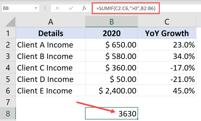
Below I have a data set where I want to add or the cells where the growth is positive which is in column C.
Below is the formula that will add only those cells in column B, where the corresponding cell in column C has a positive value:
=SUMIF(C2:C6,">0",B2:B6)
Note that this is a similar formula as we had used above (with one change). Instead of having the same ‘criteria’ and ‘sum’ range, it’s different in this formula.
Also read: SUM Based on Partial Text Match in Excel (SUMIF)
SUM Negative Numbers Only
Just like we did the sum of all the positive numbers, you can use a similar concept to sum only the negative values only.
Suppose you have the dataset as shown below and you want to sum only the negative numbers in column B.
Below is the formula to do this:
=SUMIF(B2:B8,"<0",B2:B8)
The above formula uses “<0” as the criteria (second argument), which only adds the negative numbers.
And you can use the same concepts shown earlier to add negative numbers below a specific number and can even have separate criteria and sum ranges.
So this is how you can use a simple SUMIF formula to add only the positive numbers or negative numbers in Excel.
I hope you found this tutorial useful!
Other Excel tutorials you may like:
- Change Negative Number to Positive in Excel [Remove Negative Sign]
- How to Sum Across Multiple Sheets in Excel? (3D SUM Formula)
- How to Add Plus Sign Before Numbers in Excel
- SUMPRODUCT vs SUMIFS Function in Excel
- How to Sum a Column in Excel
- How to SUM values between two dates (using SUMIFS formula)
- How To Subtract In Excel (Subtract Cells, Column, Dates/Time)
- Show Negative Numbers in Parentheses (Brackets) in Excel (Easy Ways)


What about if we would like to sum only postive or greater/smaller numbers from a list of cells like A2, A4, A6, A8, etc instead of a range of cells like A1:A9?