Change Negative Number to Positive in Excel [Remove Negative Sign]

Most of the people who work with Excel spreadsheets deal with numbers in large/small datasets.

And when you work with numbers, you will have all types of it (positive, negative, decimals, date/time).

One of the common tasks a lot of us need to do often is to convert these numbers from one format to another.

And probably the most common one is when you have to change negative numbers to positive numbers (remove the negative sign) for some calculations.

And again, there are multiple ways you can do this in Excel.

In this tutorial, I will show you some simple ways to change negative numbers to positive in Excel (using formulas, a copy-paste technique, and other awesome methods).

I’ll also show you how to hide the minus sign without changing the value, and how to do the opposite (make positive numbers negative).

So if you’re interested, keep reading!

Use the ABS function to Change all Negative Numbers to Positive

Excel has a dedicated function that strips out the negative sign and gives you the absolute value.

… the ABS function

Below I have a list of office expenses where some amounts are negative, and I want to get all of them as positive numbers in column C.

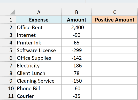
Below is the formula that will do this:

=ABS(B2:B11)

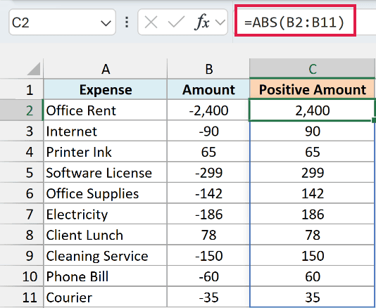
The above ABS function doesn’t impact the positive numbers but converts negative numbers into positive values.

Since I’ve given it the whole range B2:B11, you only need to enter it in cell C2. The formula spills down automatically and fills the result in C2:C11.

If you are using Excel 2019 or earlier, enter the below formula in cell C2 and then copy it down the range:

=ABS(B2)

Now that you have the required result, you can convert these formulas to values (and copy it over the original data in case you don’t need it).

Important: One minor drawback of the ABS function is that it can only work with numbers. In case you have text data in some of the cells and you use the ABS function, it will give you #VALUE! error.

If your data has some text in it, the next method handles it without any errors.

Multiply with minus 1 to Convert Negative Number to Positive

If you have a column full of numbers and you want to quickly get the numbers where negatives have been converted into positive, you can easily do that by multiplying these negative values by -1.

But you also have to ensure that you’re only multiplying the negative numbers and not the positive ones.

Below I have the same expense list, but the amount for Courier is still Pending (a text value), and I want the positive amounts in column C.

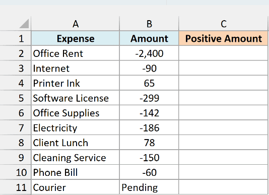
Below is the formula that will convert negative numbers to positives and keep the rest unchanged:

=IF(B2:B11<0,-B2:B11,B2:B11)

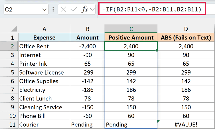
The above formula uses the IF function to first check whether the number is negative or not. If it’s negative, a minus sign is added to the reference (which is the same as multiplying it by -1), and that gives us a positive number.

If the value is not negative, the formula returns it as it is.

In case you have text values in the dataset as well, this formula is going to ignore that (and only negative values will be changed).

That’s why Pending stays as Pending in cell C11, while the ABS formula in column D gives a #VALUE! error for the same row.

One thing to keep in mind is that if a cell in your data is blank, this formula returns 0 for it.

If you are using Excel 2019 or earlier, enter the below formula in cell C2 and then copy it down the range:

=IF(B2<0,-B2,B2)

Here again, once you have the result, you can convert the formulas to values and replace the original data if you want.

Multiply Using Paste Special To Reverse the Sign

In case you want to reverse the sign of the number (i.e., change negative to positive and positive to negative), you can also use this paste special multiplication technique.

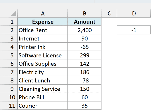
Below I have the expense list, and I want to reverse the sign of the amounts in column B.

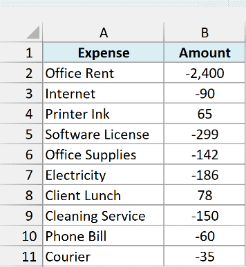
Below are the steps to reverse the sign using Paste Special:

1. In any empty cell in the worksheet, enter -1

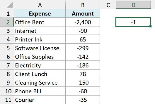
2. Copy this cell (which has the value -1)

3. Select the range where you want to reverse the sign (B2:B11 in this example)

4. Right-click on any of the selected cells

5. Click on Paste Special. This will open the Paste Special dialog box

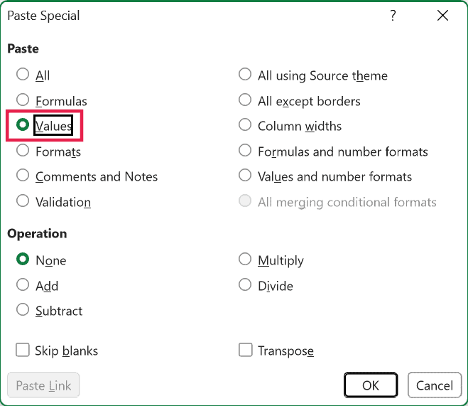
6. In the Paste options, select ‘Values’

7. In the Operation options, select ‘Multiply’

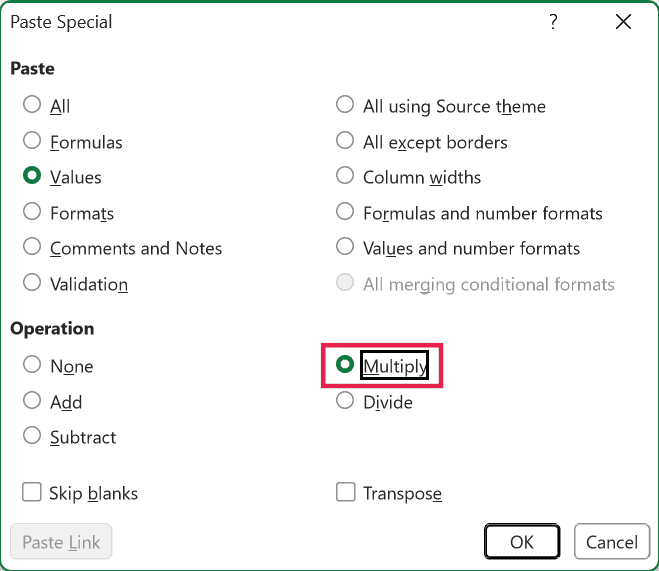
8. Click OK

9. Delete -1 from the cell

You would notice that the above steps instantly reverse the sign of the number (i.e., positive numbers become negative and negative numbers become positive).

Selecting ‘Values’ in step 6 makes sure only the multiplication happens, so the formatting of your cells stays as it is.

Important: If your selection has blank cells, Paste Special turns them into 0. So select only the cells that have numbers before you paste.

Also, if a cell has a formula, Paste Special keeps the formula and multiplies it by -1. For example, =5-10 becomes =(5-10)*-1.

But what if you only want to convert negative numbers to positive numbers and not the other way round?

In that case, you somehow first need to select all the negative numbers and then follow the above steps.

So first enter -1 in an empty cell and copy it (steps 1 and 2 above). Then select only the negative numbers, and do steps 4 to 9 on that selection.

Here is how to select only the negative numbers in Excel:

1. Select the entire dataset (the cells with the numbers)

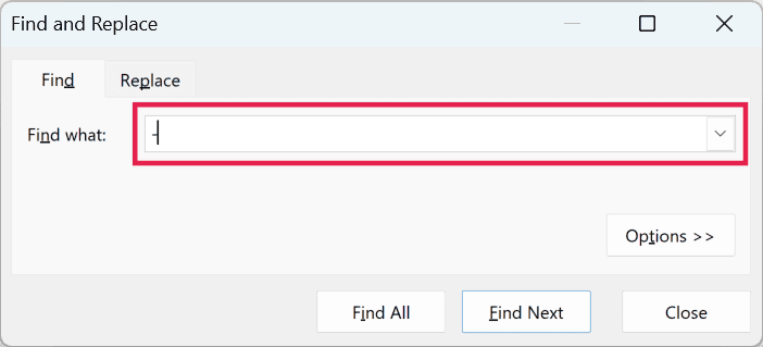
2. Hold the Control key and then press the F key. This will open the Find and Replace dialog box.

3. In the Find what field, enter – (the minus sign)

4. Click on Find All

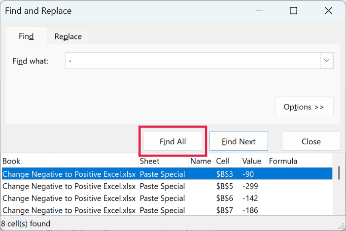
5. Hold the Control Key and press the A key.

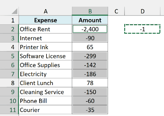
6. Close the Find and Replace dialog box

The above steps would select only those cells that have a negative sign. Now that you have these cells selected, you can use the Paste Special technique to change the sign of only the negative numbers.

Find All picks up any cell with a minus sign in it, including text like N-12 or a formula with a subtraction. That’s why it’s best to select only the cells with the numbers in step 1.

This technique has two advantages over the formula technique (the two methods covered before this):

1. It doesn’t require you to add an additional column and then use a formula to get the result in that column. You can use this on your existing dataset.
2. You don’t need to convert the formulas to values (as the result you get is already value and not a formula)

Remove the Minus Sign Using Find and Replace

If all you want is to remove the minus sign from the numbers, you can also do it with Find and Replace. Like Paste Special, this changes the numbers right where they are.

Below I have the expense list, and I want to remove the minus sign from the amounts in column B.

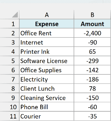
Here are the steps to remove the minus sign using Find and Replace:

1. Select the cells that have the numbers (B2:B11 in this example)

2. Hold the Control key and press the H key. This will open the Replace tab of the Find and Replace dialog box.

3. In the Find what field, enter – (the minus sign)

4. Leave the Replace with field empty

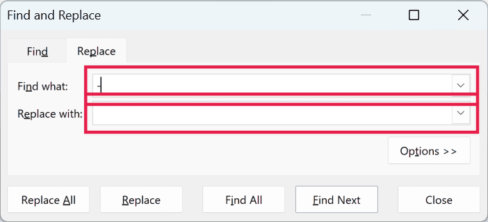
5. Click on Replace All

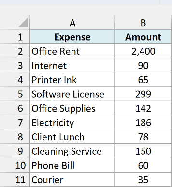
Excel removes the minus sign from every number in the selection. The values stay as numbers, so you can still use them in your calculations.

Important: Find and Replace removes every minus sign in the selection, including the ones in formulas and text. A formula like =A1-A2 becomes =A1A2 (and shows a #NAME? error), so select only the cells with the numbers before you click Replace All.

If only one cell is selected when you open Find and Replace, Excel runs the replace on the entire worksheet, which is why the selection in step 1 matters.

Hide the Negative Sign with a Custom Number Format

Sometimes, you don’t want to change the numbers at all. You just want them to show up without the minus sign (for example, in a report where it’s already clear that these are expenses).

In that case, you can use a custom number format. It changes how the number looks, while the actual value in the cell stays negative.

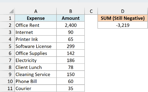
Below I have the expense list, and I want the amounts in column B to show without the minus sign.

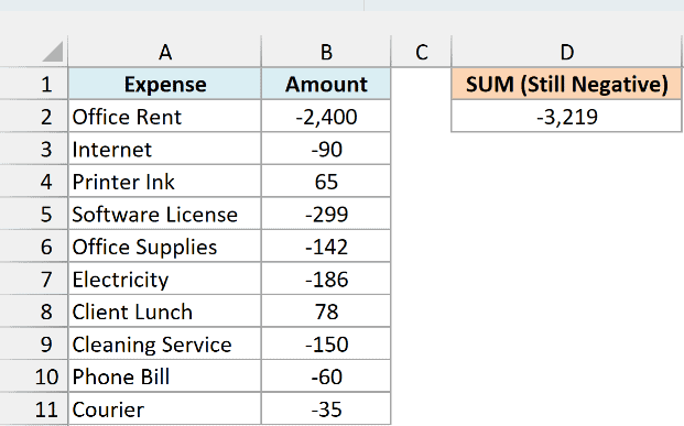
Here are the steps to hide the negative sign using a custom number format:

1. Select the cells that have the numbers (B2:B11 in this example)

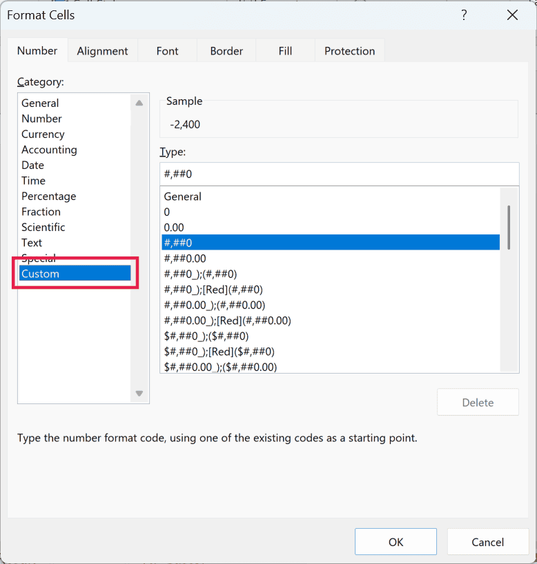
2. Hold the Control key and press the 1 key. This will open the Format Cells dialog box.

3. In the Number tab, click on Custom in the Category list

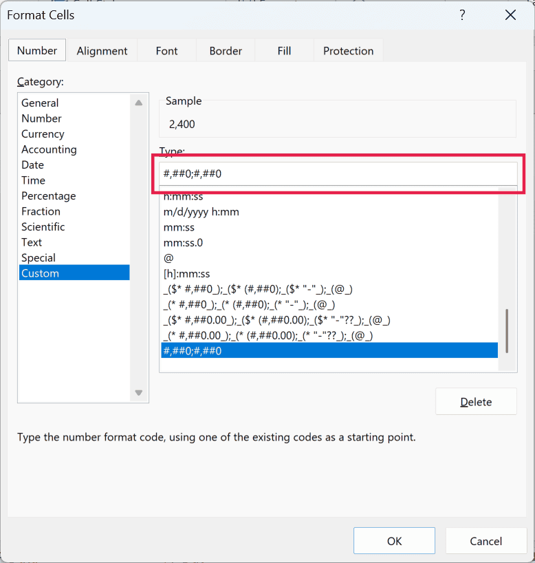
4. In the Type field, enter #,##0;#,##0

5. Click OK

A custom number format can have different parts separated by a semicolon. The first part is for positive numbers and the second part is for negative numbers, and since the second part here (#,##0) has no minus sign, negative numbers show without it.

If you want to learn more about how these format codes work, I’ve covered them in detail in my tutorial on how to show negative numbers in parentheses.

The #,##0 code shows whole numbers. If your numbers have decimals, use #,##0.00;#,##0.00 instead, because #,##0 rounds what you see (89.99 would show up as 90).

Important: This only changes how the numbers look. Any formula that uses these cells still sees the negative values, which is why the SUM formula in cell D2 still gives -3,219.

So if you need actual positive numbers for your calculations, use one of the methods covered above instead.

Flash Fill To Remove the Negative Sign

Flash Fill is a functionality that was introduced in Excel 2013.

It allows you to quickly identify patterns and then give you the result where the pattern has been applied to the entire dataset.

One use of this is when you have names and you want to separate first name and last name.

As soon as you type the first name in an adjacent cell a couple of times, Flash Fill will identify the pattern and give you all the first names.

Similarly, you can use it to quickly remove the negative sign from a number, while the positive values remain unchanged.

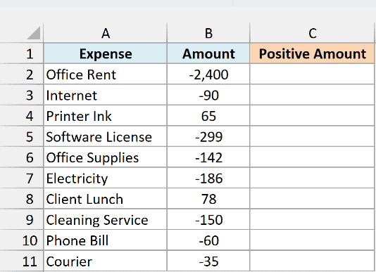
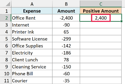
Below is a dataset where I have the negative numbers and I want to change these to positive values in column C.

Below are the steps to change negative numbers to positive numbers using Flash Fill:

1. In the cell adjacent to the one with the data, enter the expected result manually. In this example, I will manually enter 2400 in cell C2

2. Select the cell below it (C3)

3. Click the Data tab

4. Click on Flash Fill

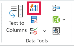
The above steps would give you the expected result, where the negative sign has been removed.

Pro Tip: Instead of going to the Data tab, you can press Control + E after step 2 to run Flash Fill.

You can also do this with the fill handle. Enter the result in C2, select it, and place the cursor over the bottom-right corner of the selection (it changes into a plus icon).

Then double-click (or click and drag down) to fill the column, click on the AutoFill Options icon that appears at the bottom-right of the filled cells, and click on Flash Fill.

One thing you need to remember when using this method is that Excel relies on guessing the pattern. So you will have to at least show Excel that you are converting a negative number to positive.

This means that you will have to manually enter the expected result until you have covered at least one negative number.

Also, Flash Fill works with what the cell shows, not with the value behind it. So if your numbers use a format like 1,234.00, it can guess the wrong pattern (for example, 64.50 can come out as 6450), so always check the results.

And since Flash Fill gives you values (not formulas), you’ll need to run it again if the original numbers change.

Use Power Query to Convert Negative Numbers to Positive

If this is something you need to do every time you get new data (say, a monthly export from your accounting software), Power Query is a good option. You set it up once, and the next time, you just refresh it.

Below I have the expense list, and I want a copy of it where all the amounts are positive.

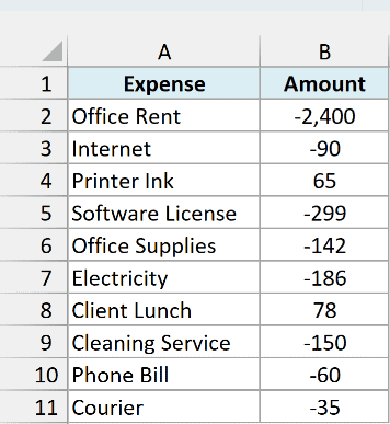
Here are the steps to convert negative numbers to positive using Power Query:

1. Select any cell in the dataset

2. Click the Data tab

3. In the Get & Transform Data group, click on From Table/Range

4. In the Create Table dialog box, make sure ‘My table has headers’ is checked and click OK

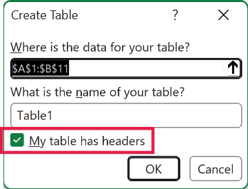
This opens the Power Query Editor with your data in it. If your data is already an Excel Table, you won’t see the Create Table dialog box, and the editor opens right away.

When the data opens in the editor, Power Query adds a Changed Type step that sets a data type for each column. Since the amounts here are whole numbers, it sets the Amount column as Whole Number.

That type stays with the query, so if you later add decimal amounts to the source table and refresh, they get rounded (89.99 comes back as 90).

So if your amounts could have decimals, fix the type now, before step 5. Click the type icon on the left of the Amount header, choose Decimal Number, and click Replace current when Power Query asks.

5. Select the Amount column by clicking on its header

6. Click the Transform tab

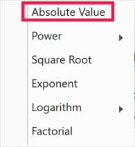
7. In the Number Column group, click on Scientific

8. Click on Absolute Value

9. Click the Home tab and click on Close & Load

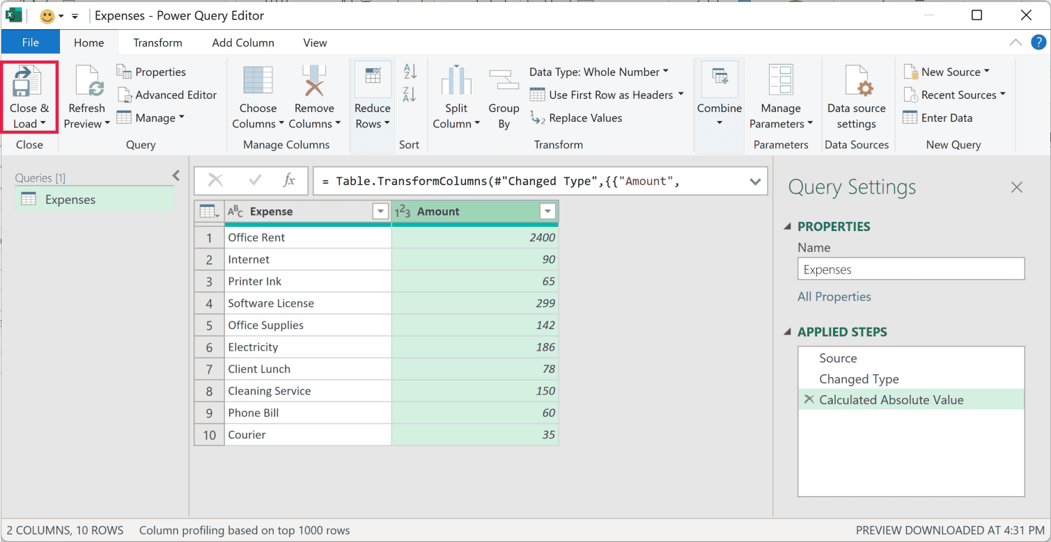
The Absolute Value command does the same thing as the ABS function. It converts every negative number in the column to positive and leaves the positive numbers as they are.

Close & Load puts the result in a new worksheet as an Excel Table. In the example file, I’ve loaded it next to the original data (using Close & Load To) so you can compare the two.

Next time you get new data, paste it into the original table, then right-click the result table and click Refresh. Power Query runs the same steps again.

Power Query is available in Excel 2016 and later versions (including Microsoft 365). In Excel 2010 and 2013, you can get it as a free add-in.

Convert Negative Numbers to Positive with a Single Click (VBA)

You can also use VBA to convert negative values to positive values.

I would recommend using this method if doing this is something you have to do often. Maybe you regularly get the dataset from a database or a colleague and you have to do this every time.

In such a case, you can create and save the VBA macro code to the Personal Macro Workbook and place the VBA in the Quick Access Toolbar.

This way, the next time you get a dataset where you have to do this, you simply select the data and click on the icon in the QAT…

… and you’ll be done!

Don’t worry, I will show you the exact steps to get this up and running.

Below is the VBA code that will convert negative values to positive values in the selected range:

Sub ChangeNegativeToPositive()
For Each Cell In Selection
    If Cell.Value < 0 Then
        Cell.Value = -Cell.Value
    End If
Next Cell
End Sub

Sub ChangeNegativeToPositive()
For Each Cell In Selection
    If Cell.Value < 0 Then
        Cell.Value = -Cell.Value
    End If
Next Cell
End Sub

The above code uses the For Next loop to go through each cell in the selection.

It uses the IF statement to check whether the cell value is negative or not. If the value is negative, the sign is reversed, and if it’s not, it’s ignored.

Text and blank cells in the selection are skipped. But if a cell has a formula that returns a negative number, the code replaces the formula with the positive value.

Also, you can’t undo the changes made by a macro with Control + Z. So it’s a good idea to save a copy of your data before you run it.

You can add this code to a regular module in a workbook (if you only want to use this in that workbook).

To do this, press Alt + F11 to open the Visual Basic Editor, click on Insert > Module, and paste the code in the module window that opens.

And in case you want to use this macro code in any workbook on your system, you can save it in a personal macro workbook.

Here are the steps to get the Personal Macro Workbook (PMW).

Here are the steps to save this code in the PMW.

Now let me show you how to add this code to the Quick Access Toolbar (steps are the same whether you save this code in a single workbook or in the PMW)

1. Open the workbook where you have the data

2. Add the VBA code to the workbook (or to the PMW)

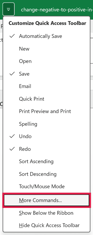
3. Click on the ‘Customize Quick Access Toolbar’ option in the QAT

If you don’t see the Quick Access Toolbar, right-click anywhere on the ribbon and click on Show Quick Access Toolbar.

4. Click on ‘More Commands’

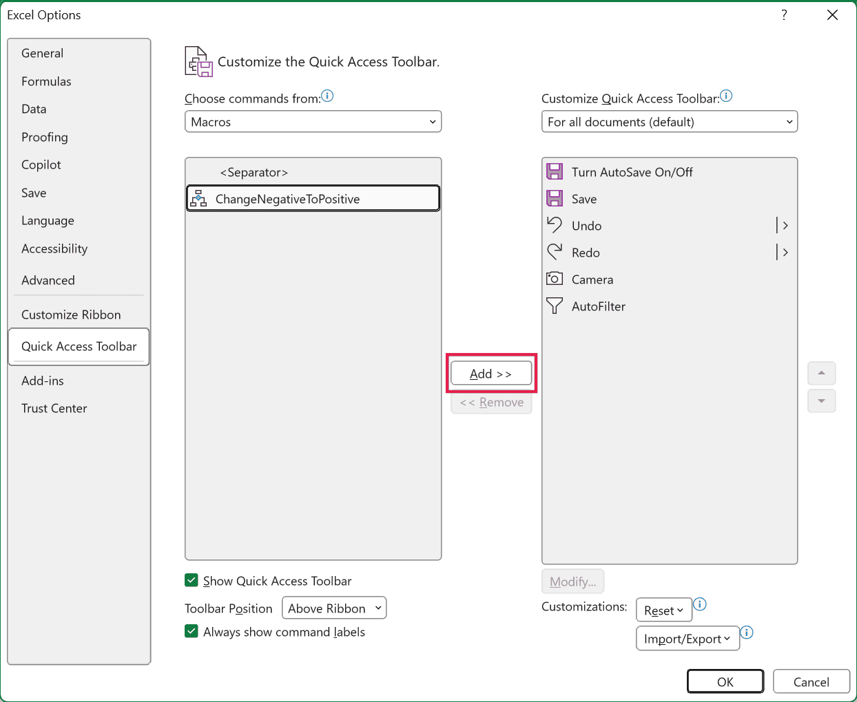
5. In the Excel Options dialog box, click on the ‘Choose commands from’ drop-down

6. Click on Macros. This will show you all the macros in the workbook (or the Personal Macro Workbook)

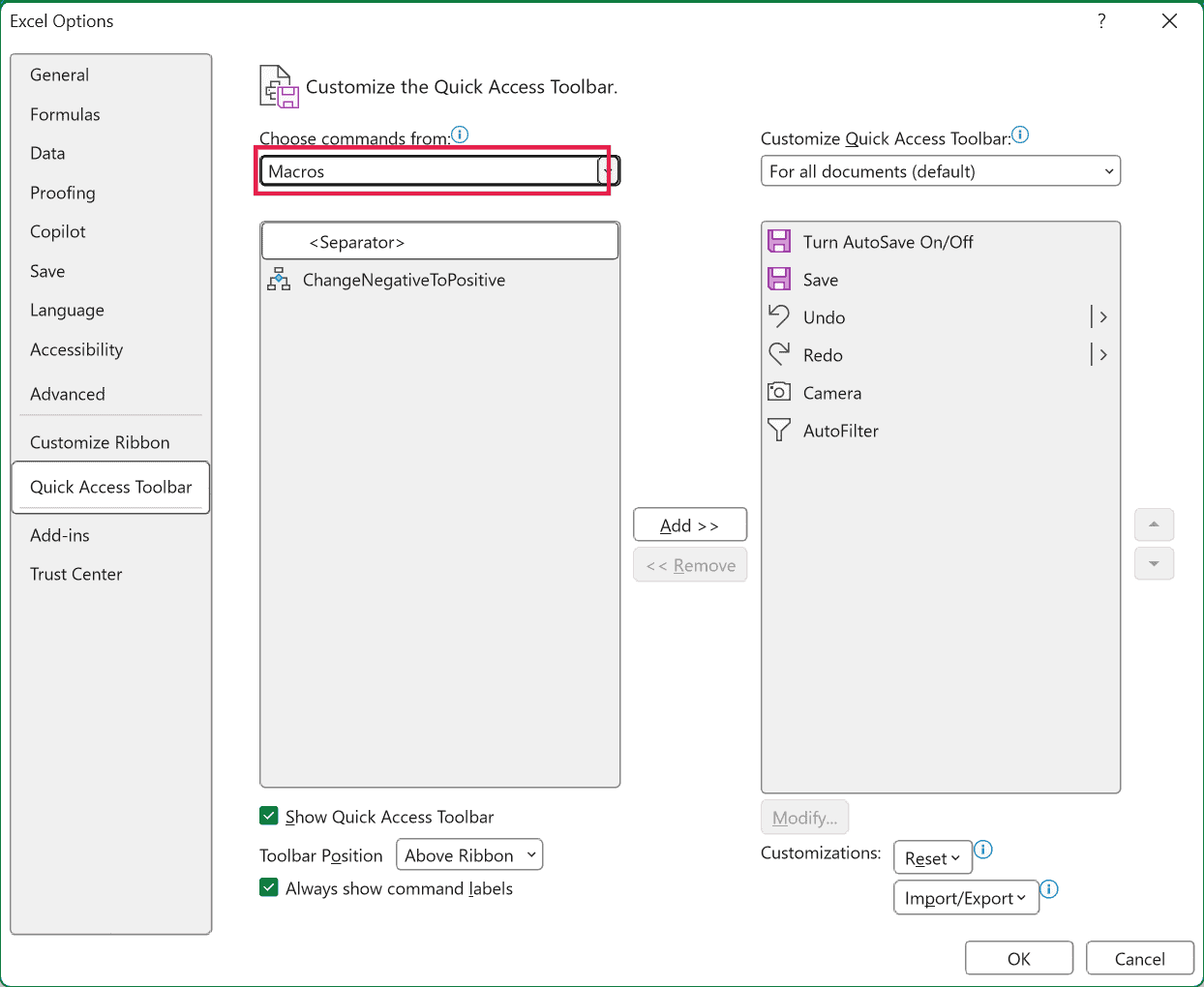
7. Select the ChangeNegativeToPositive macro

8. Click on the ‘Add’ button

9. Click OK

Now you will have the macro icon in the QAT.

To use this macro with a single click, simply make the selection and click on the macro icon.

Important: In case you’re saving the VBA macro code in the workbook, you need to save the workbook in the macro-enabled format (XLSM). Otherwise, the code is removed when you save the file.

Change Positive Numbers to Negative in Excel

And in case you need to do the opposite (make all the numbers negative), you can use a similar formula.

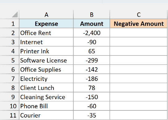
Below I have the expense list, and I want all the amounts as negative numbers in column C.

Below is the formula that will do this:

=-ABS(B2:B11)

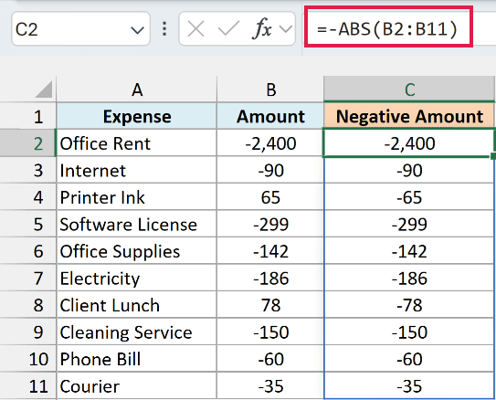
The ABS function first converts every number to positive, and the minus sign in front of it then turns it negative. So the numbers that are already negative stay negative.

If you are using Excel 2019 or earlier, enter the below formula in cell C2 and then copy it down the range:

=-ABS(B2)

If you want to flip the sign of every number instead (positive to negative and negative to positive), you can use the Paste Special method covered above.

So these are some of the ways you can change negative numbers to positive in Excel. I covered the ABS and IF formulas, Paste Special, Find and Replace, Flash Fill, Power Query, and VBA.

I also showed you how to hide the minus sign with a custom number format, and how to make positive numbers negative.

I hope you found this Excel tutorial useful.

You may also like the following Excel tutorials:

• Convert Date to Text in Excel
• How to Add Plus Sign Before Numbers in Excel
• Convert Text to Numbers in Excel
• How to add serial numbers to rows in Excel
• How to Stop Excel from Changing Numbers to Dates
• How to Sum Only Positive or Negative Numbers in Excel
• How to Make Negative Numbers Show Up in Red in Excel
• SIGN Function in Excel