
In this blog post, I will show you a formula to get a list unique items from a list in excel that has repetitions. While this can be done using Advanced Filter or Conditional Formatting, the benefit of using a formula is that it makes your unique list dynamic. This means that you continue to get a unique list even when you add more data to the original list.
Get Unique Items from a List in Excel Using Formulas
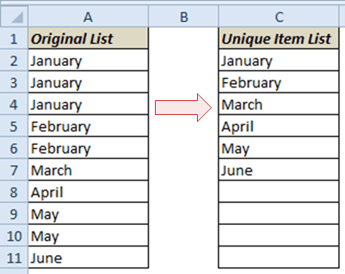
Suppose you have a list as shown above (which has repetitions) and you want to get unique items as shown on the right.
Here is a combination of INDEX, MATCH and COUNTIF formulas that can get this done:
=IFERROR(INDEX($A$2:$A$11,MATCH(0,COUNTIF($C$1:C1,$A$2:$A$11),0)),"")
How it works

When there are no more unique items, the formula displays an error. To handle it, I have used the Excel IFERROR function to replace the error message with a blank.
Since this is an array formula, use Control + Shift + Enter instead of Enter.
This is a smart way to exploit the fact that MATCH() will always return the first matching value from a range of values. For example, in this case, MATCH returns the position of the first 0, which represents the first non-matching item.
I also came up with another formula that can do the same thing (its longer but uses a smart MATCH formula trick)
=IFERROR(INDEX($A$2:$A$11,SMALL(MATCH($A$2:$A$11,$A$2:$A$11,0), SUM((COUNTIF($A$2:$A$11,$C$1:C1)))+1)),"")
I will leave it for you to decode. This is again an array formula, so use Control + Shift + Enter instead of Enter.
In case you come up with a better formula or a smart trick, do share it with me.


How can I do this without using Array Formulas? It is now slowing down my data sheet with only over 180 rows
This Formular returns always 0. What do I do wrong? Where do I use CTRL+Shift+Enter? Why?
Great post. How would the formula look if you were wanting to do the same thing (Return a list of unique values) but with the data sourced from across 2 or more columns????
This formula is not working for me, I always get ‘0’, I have dragged the formula to columns by double clicking the + sign
Hai sumit, This formula is ok for small data sets but if we need to work with a huge data set i want to know how to use the unique values generated from a pivot table in excel forumlas and functions.
But isn’t Pivot Table can do the same job easier
It can, but Pivot table is not dynamic so you need to refresh it every time there is a change in the back-end data.
In which cell this formula will go?
In this example, the formula is in C2:C11
In which cell this formula will go?
Hi Sumit i’M looking for this formula quite a long time.Great work!!. Also Created a table version of this formula using structured references and working fine and would like to share this
{=IFERROR(INDEX([Orginal List],MATCH(0,COUNTIF(OFFSET(Unique[[#Headers],[Unique Value]],ROW()-1-ROW(Unique[[#Headers],[Unique Value]]),0,ROW(Unique[[#Headers],[Unique Value]])-ROW()),[Orginal List]),0)),””)}
Where Unique is the Table name and Original List ,Unique Value are its column.
Hi Karthik.. Thanks for sharing the formula. It is almost always a good idea to convert data range into a table.
May i Get the example excel file link for this.
Hi! I have fixed the error and now the formula works well. Thanks a lot! It’s a very useful formula. But now I have two columns of data, do you know how can I combine multiple columns of data and remove the duplicates?
Hi Wang.. Glad it was helpful. In your query, do you have numbers in the 2 columns, or there is a mix of numbers and alphabets.
Also, can you create a helper (additional) column, copy paste this data to get it in one column and use this formula, or you looking for a dynamic formula?
Hi! Thanks for your reply! Yes I have numbers in 2 columns. Right now I’m doing with a helper (additional) column, but is there a dynamic formula that can do this without copy and paste?
Try this: (Assuming you have data in A2:B18)
=IFERROR(IF(ROWS($C$2:C2)<=COUNT($A$2:$B$18),INDEX($A$2:$B$18,IF(ROWS($C$2:C2)<=COUNT($A$2:$A$18),ROWS($C$2:C2),ROWS($C$2:C2)-COUNT($A$2:$A$18)),IF(ROWS($C$2:C2)<=COUNT($A$2:$A$18),1,2)),""),"")
This would give you a single column list with data from both the columns (and this is dynamic)
I am sure there could be a shorter way, but if this works for you, nothing like that.
Thanks! I think your formula would work. But actually the data are not in two adjacent columns, meaning they are in $A$1:$A$10 and $E$1:$E$10. How should I change your formula to make it work with these two column?
Try this:
=IFERROR(IF(ROWS($C$2:C2)<=COUNT($A$2:$A$18,$E$2:$E$18),INDEX($A$2:$E$18,IF(ROWS($C$2:C2)<=COUNT($A$2:$A$18),ROWS($C$2:C2),ROWS($C$2:C2)-COUNT($A$2:$A$18)),IF(ROWS($C$2:C2)<=COUNT($A$2:$A$18),1,5)),""),"")
Thanks! I’ll try it out.
Hi! This formula is exactly what I’m looking for, but I got an error with it. I attach the screenshot here. Sorry that I’m kind of new to excel..hope you can help me solve this problem..
Hello, I got the same exception. How can I fix it?
Very usefull……….
Thanks Ankur. Glad you found this useful