Find and Remove Duplicates in Excel

Watch Video – How to Find and Remove Duplicates in Excel

With a lot of data…comes a lot of duplicate data. 

Duplicates in Excel can cause a lot of troubles. Whether you import data from a database, get it from a colleague, or collate it yourself, duplicates data can always creep in. And if the data you are working with is huge, then it becomes really difficult to find and remove these duplicates in Excel.

In this tutorial, I’ll show you how to find and remove duplicates in Excel.

Find and Highlight Duplicates in Excel

Duplicates in Excel can come in many forms. You can have it in a single column or multiple columns. There may also be a duplication of an entire row.

Finding and Highlight Duplicates in a Single Column in Excel

Conditional Formatting makes it simple to highlight duplicates in Excel.

Here is how to do it:

• Select the data in which you want to highlight the duplicates.

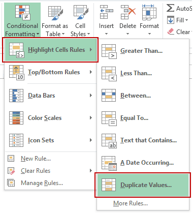
• Go to Home –> Conditional Formatting –> Highlight Cell Rules –> Duplicate Values.

• In the Duplicate Values dialog box, select Duplicate in the drop down on the left, and specify the format in which you want to highlight the duplicate values. You can choose from the ready-made format options (in the drop down on the right), or specify your own format.

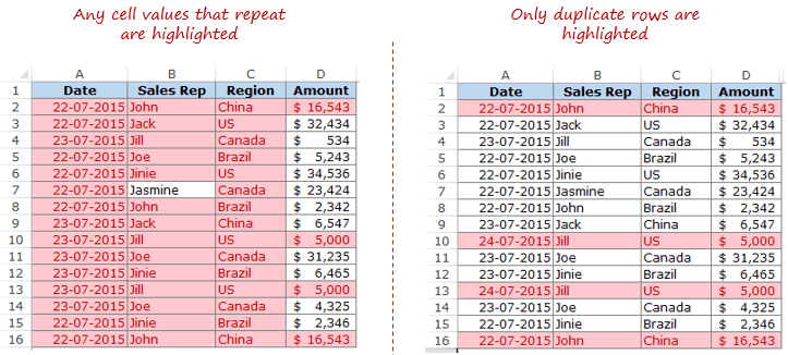
• This will highlight all the values that have duplicates.

Quick Tip: Remember to check for leading or trailing spaces. For example, “John” and “John ” are considered different as the latter has an extra space character in it. A good idea would be to use the TRIM function to clean your data.

Finding and Highlight Duplicates in Multiple Columns in Excel

If you have data that spans multiple columns and you need to look for duplicates in it, the process is exactly the same as above.

Here is how to do it:

• Select the data.
• Go to Home –> Conditional Formatting –> Highlight Cell Rules –> Duplicate Values.
• In the Duplicate Values dialog box, select Duplicate in the drop down on the left, and specify the format in which you want to highlight the duplicate values.
• This will highlight all the cells that have duplicates value in the selected data set.

Finding and Highlighting Duplicate Rows in Excel

Finding duplicate data and finding duplicate rows of data are 2 different things. Have a look:

Finding duplicate rows is a bit more complex than finding duplicate cells.

Here are the steps:

• In an adjacent column, use the following formula:
  =A2&B2&C2&D2
  Drag this down for all the rows. This formula combines all the cell values as a single string. (You can also use the CONCATENATE function to combine text strings)

By doing this, we have created a single string for each row. If there are duplicate rows in this dataset, then these strings would be exactly the same for it.

Now that we have the combined strings for each row, we can use conditional formatting to highlight duplicate strings. A highlighted string implies that the row has a duplicate.

Here are the steps to highlight duplicate strings:

• Select the range that has the combined strings (E2:E16 in this example).
• Go to Home –> Conditional Formatting –> Highlight Cell Rules –> Duplicate Values.
• In the Duplicate Values dialog box, make sure Duplicate is selected and then specify the color in which you want to highlight the duplicate values.

This would highlight the duplicate values in column E.

In the above approach, we have highlighted only the strings that we created.

But what if you want to highlight all the duplicate rows (instead of highlighting cells in one single column)?

Here are the steps to highlight duplicate rows:

• In an adjacent column, use the following formula:
  =A2&B2&C2&D2
  Drag this down for all the rows. This formula combines all the cell values as a single string.

• Select the data A2:D16.
• With the data selected, go to Home –> Conditional Formatting –> New Rule.

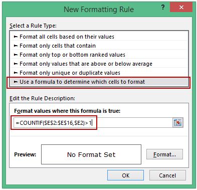
• In the ‘New Formatting Rule’ dialog box, click on ‘Use a formula to determine which cells to format’.
• In the field below, use the following COUNTIF function:
  =COUNTIF($E$2:$E$16,$E2)>1

• Select the format and click OK.

This formula would highlight all the rows that have a duplicate.

Also read: Remove Duplicates Within a Cell in Excel

Remove Duplicates in Excel

In the above section, we learned how to find and highlight duplicates in excel. In this section, I will show you how to get rid of these duplicates.

Remove Duplicates from a Single Column in Excel

If you have the data in a single column and you want to remove all the duplicates, here are the steps:

• Select the data.
• Go to Data –> Data Tools –> Remove Duplicates.
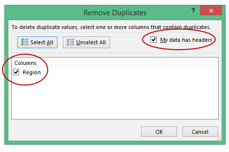
• In the Remove Duplicates dialog box:
  • If your data has headers, make sure the ‘My data has headers’ option is checked.
  • Make sure the column is selected (in this case there is only one column).

• Click OK.

This would remove all the duplicate values from the column, and you would have only the unique values.

CAUTION: This alters your data set by removing duplicates. Make sure you have a back-up of the original data set. If you want to extract the unique values at some other location, copy this dataset to that location and then use the above-mentioned steps. Alternatively, you can also use Advanced Filter to extract unique values to some other location.

Remove Duplicates from Multiple Columns in Excel

Suppose you have the data as shown below:

In the above data, row #2 and #16 have the exact same data for Sales Rep, Region, and Amount, but different dates (same is the case with row #10 and #13). This could be an entry error where the same entry has been recorded twice with different dates.

To delete the duplicate row in this case:

• Select the data.
• Go to Data –> Data Tools –> Remove Duplicates.
• In the Remove Duplicates dialog box:
  • If your data has headers, make sure the ‘My data has headers’ option is checked.
  • Select all the columns except the Date column.

• Click OK.

This would remove the 2 duplicate entries.

NOTE: This keeps the first occurrence and removes all the remaining duplicate occurrences.

Remove Duplicate Rows in Excel

To delete duplicate rows, here are the steps:

• Select the entire data.
• Go to Data –> Data Tools –> Remove Duplicates.
• In the Remove Duplicates dialog box:
  • If your data has headers, make sure the ‘My data has headers’ option is checked.
  • Select all the columns.

• Click OK.

Use the above-mentioned techniques to clean your data and get rid of duplicates.

• 10 Ways to Clean Data in Excel Spreadsheets.
• Remove Leading and Trailing Spaces in Excel.
• 24 Daily Excel Issues and their Quick Fixes.
• How to Find Merged Cells in Excel.
• Remove Duplicate Values in Excel Using VBA