When you work with data and formulas in Excel, you’re bound to encounter errors.
To handle errors, Excel has provided a useful function – the IFERROR function.
Before we get into the mechanics of using the IFERROR function in Excel, let’s first go through the different kinds of errors you can encounter when working with formulas.
Types of Errors in Excel
Knowing the errors in Excel will better equip you to identify the possible reason and the best way to handle these.
Below are the types of errors you might find in Excel.
#N/A Error
This is called the ‘Value Not Available’ error.
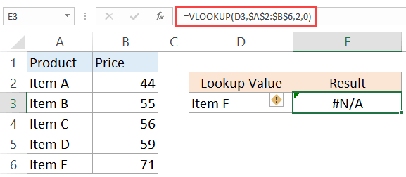
You will see this when you use a lookup formula and it can’t find the value (hence Not Available).
Below is an example where I use the VLOOKUP formula to find the price of an item, but it returns an error when it can’t find that item in the table array.

#DIV/0! Error
You’re likely to see this error when a number is divided by 0.
This is called the division error. In the below example, it gives a #DIV/0! error as the quantity value (the divisor in the formula) is 0.

#VALUE! Error
The value error occurs when you use an incorrect data type in a formula.
For example, in the below example, when I try to add cells that have numbers and character A, it gives the value error.
This happens as you can only add numeric values, but instead, I tried adding a number with a text character.

#REF! Error
This is called the reference error and you will see this when the reference in the formula is no longer valid. This could be the case when the formula refers to a cell reference and that cell reference does not exist (happens when you delete a row/column or worksheet that was referred to in the formula).
In the below example, while the original formula was =A2/B2, when I deleted Column B, all the references to it became #REF! and it also gave the #REF! error as the result of the formula.

#NAME ERROR
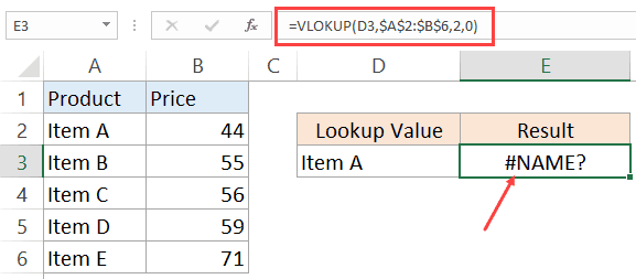
This error is likely to a result of a misspelled function.
For example, if instead of VLOOKUP, you by mistake use VLOKUP, it will give a name error.

#NUM ERROR
Num error can occur if you try and calculate a very large value in Excel. For example, =187^549 will return a number error.

Another situation where you can get the NUM error is when you give a non-valid number argument to a formula. For example, if you’re calculating the Square Root if a number and you give a negative number as the argument, it will return a number error.
For example, in the case of Square Root function, if you give a negative number as the argument, it will return a number error (as shown below).
While I have shown only a couple of examples here, there can be many other reasons that can lead to errors in Excel. When you get errors in Excel, you can’t just leave it there. If the data is further used in calculations, you need to make sure the errors are handled the right way.
Excel IFERROR function is a great way to handle all types of errors in Excel.
Excel IFERROR Function – An Overview
Using the IFERROR function, you can specify what you want the formula to return instead of the error. If the formula does not return an error, then its own result is returned.

IFERROR Function Syntax
=IFERROR(value, value_if_error)
Input Arguments
- value – this is the argument that is checked for the error. In most cases, it is either a formula or a cell reference.
- value_if_error – this is the value that is returned if there is an error. The following error types evaluated: #N/A, #REF!, #DIV/0!, #VALUE!, #NUM!, #NAME?, and #NULL!.
Additional Notes:
- If you use “” as the value_if_error argument, the cell displays nothing in case of an error.
- If the value or value_if_error argument refers to an empty cell, it is treated as an empty string value by the Excel IFERROR function.
- If the value argument is an array formula, IFERROR will return an array of results for each item in the range specified in value.
Excel IFERROR Function – Examples
Here are three examples of using IFERROR function in Excel.
Example 1 – Return Blank Cell Instead of Error
If you have functions that may return an error, you can wrap it within the IFERROR function and specify blank as the value to return in case of an error.
In the example shown below, the result in D4 is the #DIV/0! error as the divisor is 0.

In this case, you can use the following formula to return blank instead of the ugly DIV error.
=IFERROR(A1/A2,””)

This IFERROR function would check whether the calculation leads to an error. If it does, it simply returns a blank as specified in the formula.
Here, you can also specify any other string or formula to display instead of the blank.
For example, the below formula would return the text “Error”, instead of the blank cell.
=IFERROR(A1/A2,”Error”)

Note: If you are using Excel 2003 or a prior version, you will not find the IFERROR function in it. In such cases, you need to use the combination of IF function and ISERROR function.
Example 2 – Return ‘Not Found’ when VLOOKUP Can’t Find a Value
When you use the Excel VLOOKUP Function, and it can’t find the lookup value in the specified range, it would return the #N/A error.
For example, below is a data set of student names and their marks. I have used the VLOOKUP function to fetch the marks of three students (in D2, D3, and D4).

While the VLOOKUP formula in the above example finds the names of first two students, it can’t find Josh’s name on the list and hence it returns the #N/A error.
Here, we can use the IFERROR function to return a blank or some meaningful text instead of the error.
Below is the formula that will return ‘Not Found’ instead of the error.
=IFERROR(VLOOKUP(D2,$A$2:$B$12,2,0),”Not Found”)

Note that you can also use IFNA instead of IFERROR with VLOOKUP. While IFERROR would treat all kinds of error values, IFNA would only work on the #N/A errors and wouldn’t work with other errors.
Example 3 – Return 0 in case of an Error
If you don’t specify the value to return by IFERROR in the case of an error, it would automatically return 0.
For example, if I divide 100 with 0 as shown below, it would return an error.

However, if I use the below IFERROR function, it would return a 0 instead. Note that you still need to use a comma after the first argument.

Example 4 – Using Nested IFERROR with VLOOKUP
Sometimes when using VLOOKUP, you may have to look through the fragmented table of arrays. For example, suppose you have the sales transaction records in 2 separate worksheets and you want to look-up an item number and see it’s value.
Doing this requires using nested IFERROR with VLOOKUP.
Suppose you have a dataset as shown below:

In this case, to find the score for Grace, you need to use the below nested IFERROR formula:
=IFERROR(VLOOKUP(G3,$A$2:$B$5,2,0),IFERROR(VLOOKUP(G3,$D$2:$E$5,2,0),"Not Found"))
This kind of formula nesting ensure that you get the value from either of the table and any error returned is handled.
Note that in case the tables are on the same worksheet, however, in a real-life example, it likely to be on different worksheets.
Excel IFERROR Function – VIDEO
Related Excel Functions:
- Excel AND Function.
- Excel OR Function.
- Excel NOT Function.
- Excel IF Function.
- Excel IFS Function.
- Excel FALSE Function.
- Excel TRUE Function.
You May Also Like the Following Excel Tutorials:


