Use IFERROR with VLOOKUP to Get Rid of #N/A Errors

When using the VLOOKUP formula in Excel, sometimes you may end up with the ugly #N/A error. This happens when your formula can not find the lookup value.

In this tutorial, I will show you different ways to use IFERROR with VLOOKUP to handle these #N/A errors cropping up in your worksheet.

Using the combination of IFERROR with VLOOKUP allows you to show something meaningful in place of the #N/A error (or any other error for that matter).

I’ll also show you when the IFNA function is the better choice, and how the XLOOKUP function handles this without IFERROR at all.

Before getting into details on using this combination, let’s first quickly go through the IFERROR function and see how it works.

IFERROR Function Explained

With IFERROR function, you can specify what should happen in case a formula or a cell reference returns an error.

Here is the syntax of the IFERROR function.

=IFERROR(value, value_if_error)

• value: this is the argument that is checked for the error. In most cases, it is either a formula or a cell reference. When using VLOOKUP with IFERROR, the VLOOKUP formula would be this argument. If there’s no error, IFERROR returns the result of this argument as it is.
• value_if_error: this is the value that is returned if there is an error. The following error types are evaluated: #N/A, #REF!, #DIV/0!, #VALUE!, #NUM!, #NAME?, and #NULL!.

The IFERROR function works in all current Excel versions, including 365, 2024, 2021, 2019, 2016, Mac, and the web.

Possible Causes Of VLOOKUP Returning a #N/A Error

VLOOKUP function may return a #N/A error due to any of the following reasons:

1. The lookup value is not found in the lookup array.
2. There is a leading, trailing, or double space in the lookup value (or in the table array).
3. There is a spelling error in the lookup value or the values in the lookup array.

You can handle all these causes of error with the combination of IFERROR and VLOOKUP. However, you should keep an eye out for cause #2 and #3, and correct these in the source data instead of letting IFERROR handle these.

With a stray space or a spelling error, the formula shows your replacement text for a value that’s really in the list, so the real problem stays hidden.

You can treat leading, trailing, and double spaces using the TRIM function.

These three causes aren’t the only ones (numbers stored as text is another common one). If the value is clearly in your list and you still get the error, go through these 10 common fixes for VLOOKUP not working before you wrap the formula in IFERROR.

Also, #N/A isn’t the only error that IFERROR catches. It replaces other errors such as #REF! too, and that’s where the IFNA function comes in.

Note: IFERROR would treat an error irrespective of what caused it. If you only want to treat the errors caused by VLOOKUP not being able to find the lookup value, use IFNA instead.

That will make sure that errors other than #N/A are not treated and you can investigate these other errors.

IFNA would still hide a space or spelling problem though, because those return #N/A too.

Replacing VLOOKUP #N/A Error with Meaningful Text

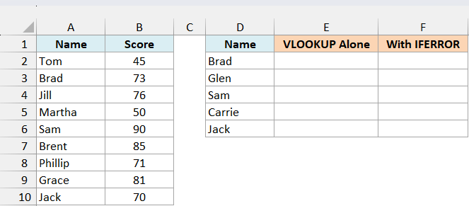
Suppose you have a dataset as shown below, with student names and their scores in columns A and B, and I want to get the score for each name in column D using a formula in column E.

The formulas in this section look up all the names at once, which needs Excel 365, 2024, or 2021. If you have an older version, the IFERROR formula you need is further down.

Here is the plain VLOOKUP formula, which I’ve entered in cell E2:

=VLOOKUP(D2:D6,$A$2:$B$10,2,FALSE)

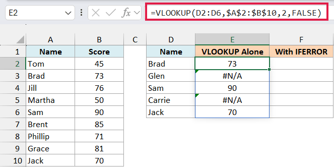
As you can see that the VLOOKUP formula returns an error for Glen and Carrie, as these lookup values are not in the list. There’s no need to copy this formula down, because it looks up all five names and spills the results by itself.

While this is a very small dataset, you may get huge datasets where you have to check the occurrence of many items. For every case when the value is not found, you will get a #N/A error.

Here is the formula you can use to get something meaningful instead of the #N/A error, entered in cell F2:

=IFERROR(VLOOKUP(D2:D6,$A$2:$B$10,2,FALSE),"Not Found")

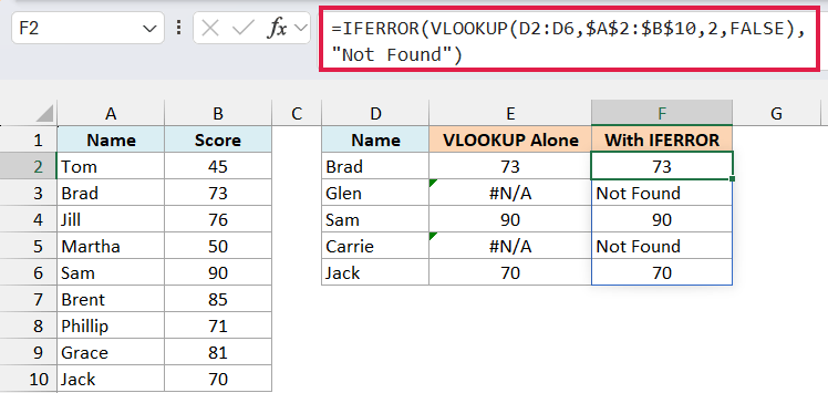
The above formula returns the text “Not Found” instead of the #N/A error. IFERROR takes each result from VLOOKUP, keeps it if it’s a real score, and swaps it for your text if it’s an error.

The cells below the formula need to be empty, otherwise you’ll get a #SPILL! error.

If you are using Excel 2019 or earlier, enter the below formula in cell F2 and then copy it down the range:

=IFERROR(VLOOKUP(D2,$A$2:$B$10,2,FALSE),"Not Found")

The dollar signs keep the table range fixed as you copy the formula, while D2 changes to D3, D4, and so on.

You can also use the same formula to return blank, zero, or any other meaningful text.

If you have Excel 365, 2024, or 2021, you can also do this without IFERROR at all, and I’ve covered that in the XLOOKUP section below.

Return Blank or 0 Instead of the VLOOKUP #N/A Error

Text like “Not Found” isn’t always what you want, so let’s see how to show a blank or a 0 instead.

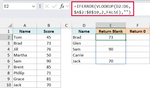
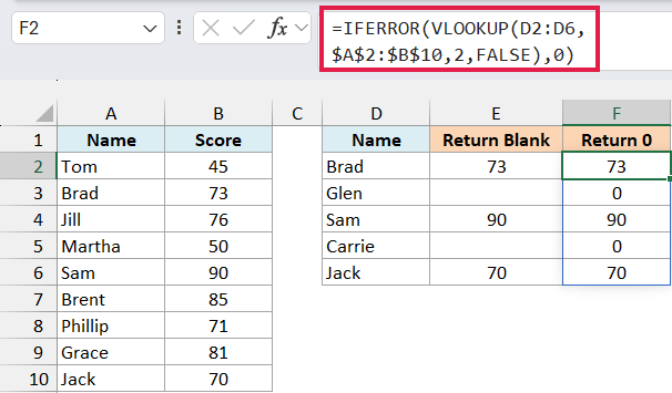
Below is the same student list, and I want to get the score for each name in column D, with a blank in column E or a 0 in column F when the name isn’t found.

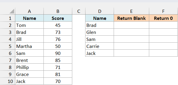
Here is the formula that shows a blank when the name is not found. The two double quotes at the end are what make the cell look empty.

=IFERROR(VLOOKUP(D2:D6,$A$2:$B$10,2,FALSE),"")

And here is the formula that shows a 0 instead:

=IFERROR(VLOOKUP(D2:D6,$A$2:$B$10,2,FALSE),0)

If you are using Excel 2019 or earlier, enter the below formula in cell E2 to show a blank, and then copy it down the range:

=IFERROR(VLOOKUP(D2,$A$2:$B$10,2,FALSE),"")

To show a 0 instead, enter the below formula in cell F2 and then copy it down the range:

=IFERROR(VLOOKUP(D2,$A$2:$B$10,2,FALSE),0)

These two options look similar, but they behave very differently once you do math on the results. To show this, I’ve added two check rows below the results.

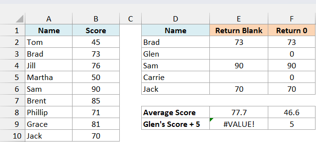
The two double quotes give you an empty text string, not a truly empty cell, and Excel can’t add a number to text. So =E3+5 tries to add 5 to Glen’s blank and returns a #VALUE! error, while =F3+5 returns 5.

That 5 has its own problem, because a 0 counts as a real score. =AVERAGE(F2:F6) returns 46.6 because Glen and Carrie are averaged in as zeros, while =AVERAGE(E2:E6) returns 77.7 because the AVERAGE function ignores the blank text cells.

So a blank is the better choice when a missing name shouldn’t count as a score, and a 0 is safer when later formulas add or subtract from these cells and a missing name really can count as zero.

Nesting VLOOKUP With IFERROR Function

In case you are using VLOOKUP and your lookup table is fragmented on the same worksheet or different worksheets, you need to check the VLOOKUP value through all of these tables.

For example, in the dataset shown below, there are two separate tables of student names and the scores, and I want to get the score for each name in column G using a formula in column H.

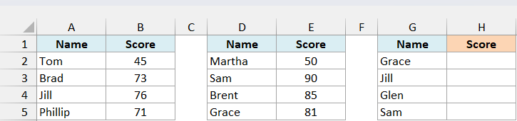
If I have to find the score of Grace in this dataset, I need to use the VLOOKUP function to check the first table, and if the value is not found in it, then check the second table.

Here is the nested IFERROR formula I can use to look for the value, entered in cell H2:

=IFERROR(VLOOKUP(G2:G5,$A$2:$B$5,2,FALSE),IFERROR(VLOOKUP(G2:G5,$D$2:$E$5,2,FALSE),"Not Found"))

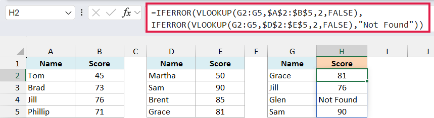
How this formula works:

• VLOOKUP(G2:G5,$A$2:$B$5,2,FALSE) looks for each name in the first table. Jill is there, so her score of 76 comes back straight away.
• The outer IFERROR steps in when a name isn’t in the first table. Instead of showing an error, it moves on to its second part, which is another IFERROR.
• VLOOKUP(G2:G5,$D$2:$E$5,2,FALSE) then checks the second table. Grace and Sam are there, so you get 81 and 90.
• “Not Found” is what’s left when a name is in neither table, which is what happens with Glen.

If you have more than two tables, keep adding one more IFERROR and VLOOKUP pair inside the formula for each extra table.

If you are using Excel 2019 or earlier, enter the below formula in cell H2 and then copy it down the range:

=IFERROR(VLOOKUP(G2,$A$2:$B$5,2,FALSE),IFERROR(VLOOKUP(G2,$D$2:$E$5,2,FALSE),"Not Found"))

IFERROR with VLOOKUP from Another Sheet

The same nesting works when your tables are on different worksheets.

In the example file, the students are split across two sheets named Class A and Class B, and on the Different Sheets tab, I want to get the score for each name in column A using a formula in column B.

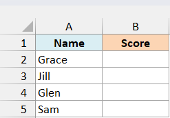
Here is the formula, entered in cell B2 of the Different Sheets tab:

=IFERROR(VLOOKUP(A2:A5,'Class A'!$A$2:$B$5,2,FALSE),IFERROR(VLOOKUP(A2:A5,'Class B'!$A$2:$B$5,2,FALSE),"Not Found"))

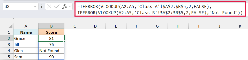
It works just like the formula in the previous section, except that each table reference now starts with its sheet name. The single quotes are there because these sheet names have a space in them.

If you are using Excel 2019 or earlier, enter the below formula in cell B2 and then copy it down the range:

=IFERROR(VLOOKUP(A2,'Class A'!$A$2:$B$5,2,FALSE),IFERROR(VLOOKUP(A2,'Class B'!$A$2:$B$5,2,FALSE),"Not Found"))

Using VLOOKUP with IF and ISERROR (Versions prior to Excel 2007)

IFERROR function was introduced in Excel 2007 for Windows. If you’re using the prior versions, then IFERROR function will not work in your system.

You can replicate the functionality of IFERROR function by using the combination of the IF function and the ISERROR function. You may also run into this combination in older workbooks, so it’s useful to know what it does.

Let me quickly show you how to use the combination of IF and ISERROR instead of IFERROR. Below is the same student list, and I want to get the score for each name in column D using a formula in column E.

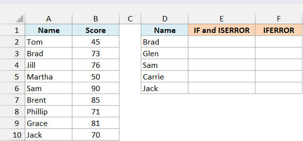
Enter the below formula in cell E2 and then copy it down the range:

=IF(ISERROR(VLOOKUP(D2,$A$2:$B$10,2,FALSE)),"Not Found",VLOOKUP(D2,$A$2:$B$10,2,FALSE))

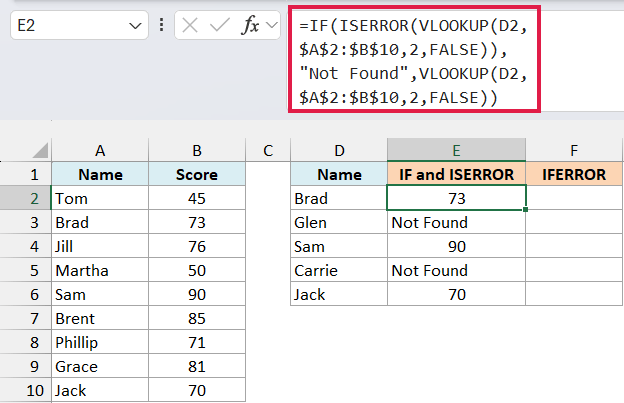
The ISERROR part of the formula checks for the errors (including the #N/A error) and returns TRUE if an error is found and FALSE if not.

• If it’s TRUE (which means that there is an error), the IF function returns the specified value (“Not Found” in this case).
• If it’s FALSE (which means that there is no error), the IF function returns the result of the VLOOKUP.

Here is the same lookup using IFERROR, entered in cell F2 and copied down:

=IFERROR(VLOOKUP(D2,$A$2:$B$10,2,FALSE),"Not Found")

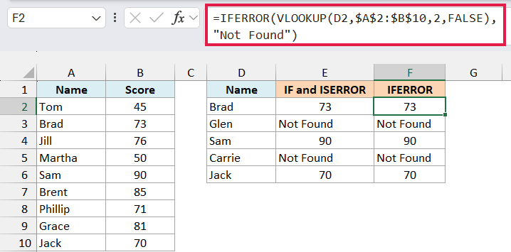
Both formulas return the same results. The IFERROR version is shorter, because you only write the VLOOKUP once.

IFERROR Vs IFNA

IFERROR treats all kinds of errors while IFNA treats only the #N/A error. When handling errors caused by VLOOKUP, you need to make sure you’re using the right formula.

Use IFERROR when you want to treat all kinds of errors. Now an error can be caused by various factors (such as the wrong formula, misspelled named range, not finding the lookup value, and returning error value from the lookup table).

It wouldn’t matter to IFERROR and it would replace all these errors with the specified value.

Use IFNA when you want to treat only #N/A errors, which are more likely to be caused by VLOOKUP formula not being able to find the lookup value.

Let’s see the difference with the same student list, where I want to get the score for each name in column D using the formulas in columns E, F, and G. The IFNA function needs Excel 2013 or later.

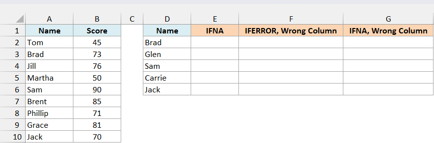
Here is the formula using IFNA, entered in cell E2:

=IFNA(VLOOKUP(D2:D6,$A$2:$B$10,2,FALSE),"Not Found")

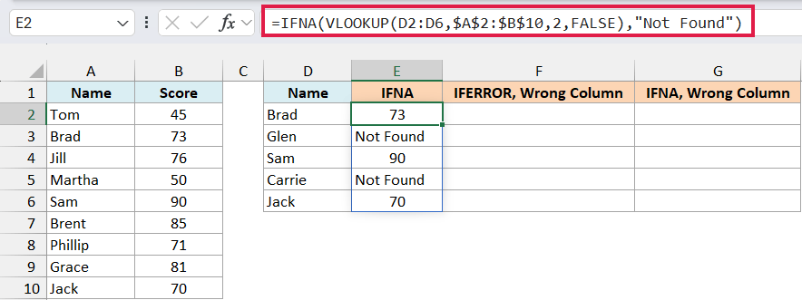
When the formula is correct, it returns the same results as IFERROR. The difference shows up when something else is wrong with your formula, so let’s say I type 3 as the column number by mistake, even though the table only has two columns.

Here is that mistake wrapped in IFERROR, entered in cell F2:

=IFERROR(VLOOKUP(D2:D6,$A$2:$B$10,3,FALSE),"Not Found")

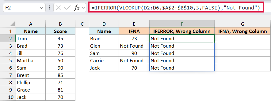
Every name in column F now shows “Not Found”, including Brad, Sam, and Jack, who are in the list. The formula is broken, but nothing on the sheet tells you that.

Here is the same mistake wrapped in IFNA, entered in cell G2:

=IFNA(VLOOKUP(D2:D6,$A$2:$B$10,3,FALSE),"Not Found")

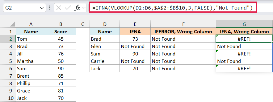
Now Brad, Sam, and Jack show a #REF! error in column G, which is your signal that the column number is wrong. Glen and Carrie still show “Not Found”, because VLOOKUP can’t find these names and returns #N/A, the one error IFNA replaces.

If you are using Excel 2013, 2016, or 2019, enter the below correct IFNA formula in cell E2 and then copy it down the range:

=IFNA(VLOOKUP(D2,$A$2:$B$10,2,FALSE),"Not Found")

Using XLOOKUP Instead of IFERROR with VLOOKUP

If you have a newer version of Excel, you may not need a wrapper at all. Below is the same student list, and I want to get the score for each name in column D using a formula in column E.

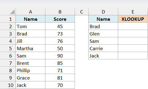
Here is the formula using the XLOOKUP function:

=XLOOKUP(D2:D6,$A$2:$A$10,$B$2:$B$10,"Not Found")

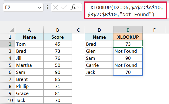
The last argument is what XLOOKUP shows when it can’t find a match, so there’s no IFERROR or IFNA around it. It only steps in for a missing match, so like IFNA, it won’t hide other mistakes in your formula.

XLOOKUP is only available in Excel 365, 2024, and 2021. I think it’s far better than VLOOKUP, and you should move to it when your Excel version and sharing requirements allow it.

VLOOKUP still makes sense when a workbook must work in an older version that does not support XLOOKUP. If you want the full comparison, here’s VLOOKUP vs XLOOKUP.

So these are the different ways you can use IFERROR with VLOOKUP to get rid of #N/A errors. Just keep in mind that IFERROR hides every error, so make sure the formula is right before you wrap it.

I hope you found this Excel tutorial useful.

You May Also Find the Following Excel Tutorials Useful:

• How to make VLOOKUP Case Sensitive.
• VLOOKUP Vs. INDEX/MATCH – The Debate Ends Here!
• Use VLookup to Get the Last Number in a List in Excel.
• How to Use VLOOKUP with Multiple Criteria
• #NAME Error in Excel – What Causes it and How to Fix it!
• Using VLOOKUP From Another Sheet in VBA
• ISNA function
• How to Get Rid of #DIV/0! Error in Excel? Easy Formulas!
• ERROR.TYPE Function in Excel