How to make VLOOKUP Case Sensitive

By default, the lookup value in the VLOOKUP function is not case sensitive. For example, if your lookup value is MATT, matt, or Matt, it’s all the same for the VLOOKUP function. It’ll return the first matching value irrespective of the case.

Making VLOOKUP Case Sensitive

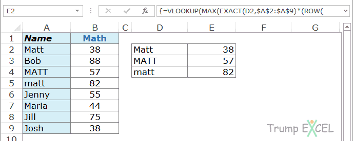
Suppose you have the data as shown below:

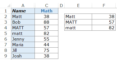
As you can see, there are three cells with the same name (A2, A4, and A5) but with a different letter case. On the right (in E2:F4), we have the three names (Matt, MATT, and matt) along with their scores in Math.

Excel VLOOKUP function is not equipped to handle case-sensitive lookup values. In this above example, no matter what lookup value case is (Matt, MATT, or matt), it’ll always return 38 (which is the first matching value).

In this tutorial, you’ll learn how to make VLOOKUP case sensitive by:

• Using a Helper Column.
• Without Using a Helper Column and Using a Formula.

Making VLOOKUP Case Sensitive – Using Helper Column

A helper column can be used to get unique lookup value for each item in the lookup array. That helps in differentiating between names with different letter case.

Here are the steps to do this:

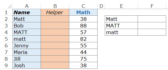
• Insert a helper column to the left of the column from where you want to fetch the data. In the example below, you need to insert the helper column between column A and C.
  
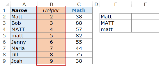
• In the helper column, enter the formula =ROW(). It’ll insert the row number in each cell.
• Use the following formula in cell F2 to get the case-sensitive lookup result.

  =VLOOKUP(MAX(EXACT(E2,$A$2:$A$9)*(ROW($A$2:$A$9))),$B$2:$C$9,2,0)

• Copy paste it for the remaining cells (F3 and F4).
  

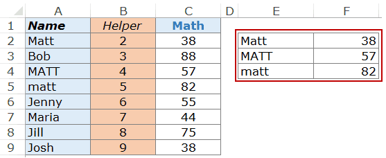
Note: Since this is an array formula, use Control + Shift + Enter instead of just enter.

How does this work?

Let’s break down the formula to understand how it works:

• EXACT(E2,$A$2:$A$9) – This part compares the lookup value in E2 with all the values in A2:A9. It returns an array of TRUEs/FALSEs where TRUE is returned when there is an exact match. In this case, where the value in E2 is Matt, it would return the following array:
  {TRUE;FALSE;FALSE;FALSE;FALSE;FALSE;FALSE;FALSE}.
• EXACT(E2,$A$2:$A$9)*(ROW($A$2:$A$9) – This part multiplies the array of TRUEs/FALSEs with the row number of A2:A9. Wherever there is a TRUE, it gives the row number, else it gives 0. In this case, it would return {2;0;0;0;0;0;0;0}.
• MAX(EXACT(E2,$A$2:$A$9)*(ROW($A$2:$A$9))) – This part returns the maximum value from the array of numbers. In this case, it would return 2 (which is the row number where there is an exact match).
• Now we simply use this number as the lookup value and use the lookup array as B2:C9.

Note: You can insert the helper column anywhere in the data set. Just make sure it is to the left of the column from where you want to fetch the data. You need to then adjust the column number in the VLOOKUP function accordingly.

Now if you’re not a fan of helper column, you can also do a case-sensitive lookup without the helper column.

Making VLOOKUP Case Sensitive – Without the Helper Column

Even when you don’t want to use the helper column, you still need to have a virtual helper column. This virtual column is not a part of the worksheet but is constructed within the formula (as shown below).

Here is the formula that’ll give you the result without the helper column:

=VLOOKUP(MAX(EXACT(D2,$A$2:$A$9)*(ROW($A$2:$A$9))),CHOOSE({1,2},ROW($A$2:$A$9),$B$2:$B$9),2,0)

How does this work?

The formula also uses the concept of a helper column. The difference is that instead of putting the helper column in the worksheet, consider it as virtual helper data that is a part of the formula.

Here is the part that works as the helper data (highlighted in orange):

=VLOOKUP(MAX(EXACT(D2,$A$2:$A$9)*(ROW($A$2:$A$9))),CHOOSE({1,2},ROW($A$2:$A$9),$B$2:$B$9),2,0)

Let me show you what I mean by virtual helper data.

In the above illustration, as I select the CHOOSE part of the formula and press F9, it shows the result that the CHOOSE formula would give.

The result is {2,38;3,88;4,57;5,82;6,55;7,44;8,75;9,38}

It’s an array where a comma represents next cell in the same row and semicolon represents that the following data is in the next row. Hence, this formula creates 2 columns of data – One column has the row number and one has the math score.

Now, when you use the VLOOKUP function, it simply looks for the lookup value in the first column (of this virtual 2 column data) and returns the corresponding score. The lookup value here is a number that we get from the combination of MAX and EXACT function.

Download the Example File

Is there any other way you know to do this? If yes, do share with me in the comments section.

You May Also Like the Following VLOOKUP Tutorials: 

• Using VLOOKUP Function with Multiple Criteria.
• Using VLOOKUP Function to Get the Last Number in a List.
• VLOOKUP Vs. INDEX/MATCH
• Use IFERROR with VLOOKUP to Get Rid of #N/A Errors.