How to Use VLOOKUP with Multiple Criteria

Watch Video – How to Use VLOOKUP Function with Multiple Criteria

Excel VLOOKUP function, in its basic form, can look for one lookup value and return the corresponding value from the specified row.

But often there is a need to use the Excel VLOOKUP with multiple criteria.

How to Use VLOOKUP with Multiple Criteria

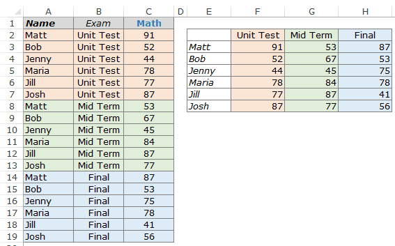
Suppose you have a data with students name, exam type, and the Math score (as shown below):

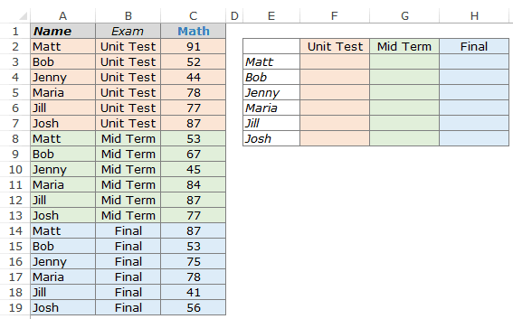
Using the VLOOKUP function to get the Math score for each student for respective exam levels could be a challenge.

One can argue that a better option would be to restructure the data set or use a Pivot Table. If that works for you, nothing like that. But in many cases, you are stuck with the data that you have and pivot table may not be an option.

In such cases, this tutorial is for you.

Now there are two ways you can get the lookup value using VLOOKUP with multiple criteria.

• Using a Helper Column.
• Using the CHOOSE function.

VLOOKUP with Multiple Criteria – Using a Helper Column

I am a fan of helper columns in Excel.

I find two significant advantages of using helper columns over array formulas:

• It makes it easy to understand what’s going on in the worksheet.
• It makes it faster as compared with the array functions (noticeable in large data sets).

Now, don’t get me wrong. I am not against array formulas. I love the amazing things can be done with array formulas. It’s just that I save them for special occasions when all other options are of no help.

Coming back to the question in point, the helper column is needed to create a unique qualifier. This unique qualifier can then be used to lookup the correct value. For example, there are three Matt in the data, but there is only one combination of Matt and Unit Test or Matt and Mid-Term.

Here are the steps:

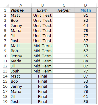
• Insert a Helper Column between column B and C.
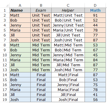
• Use the following formula in the helper column:=A2&”|”&B2
  • This would create unique qualifiers for each instance as shown below.
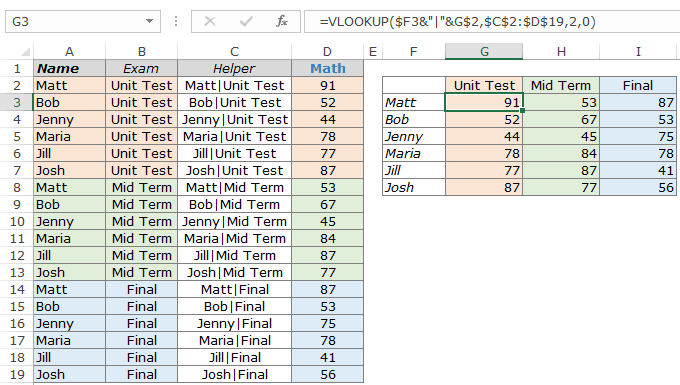
• Use the following formula in G3 =VLOOKUP($F3&”|”&G$2,$C$2:$D$19,2,0)
• Copy for all the cells.

How does this work?

We create unique qualifiers for each instance of a name and the exam. In the VLOOKUP function used here, the lookup value was modified to $F3&”|”&G$2 so that both the lookup criteria are combined and are used as a single lookup value. For example, the lookup value for the VLOOKUP function in G2 is Matt|Unit Test. Now this lookup value is used to get the score from C2:D19.

Clarifications:

There are a couple of questions that are likely to come to your mind, so I thought I will try and answer it here:

• Why have I used | symbol while joining the two criteria? – In some exceptionally rare (but possible) conditions, you may have two criteria that are different but ends up giving the same result when combined. Here is a very simple example (forgive me for my lack of creativity here):

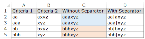
Note that while A2 and A3 are different and B2 and B3 are different, the combinations end up being the same. But if you use a separator, then even the combination would be different (D2 and D3).

• Why did I insert the helper column between column B and C and not in the extreme left? – There is no harm in inserting the helper column to the extreme left. In fact, if you don’t want to temper with the original data, that should be the way to go. I did it as it makes me use less number of cells in the VLOOKUP function. Instead of having 4 columns in the table array, I could manage with only 2 columns. But that’s just me.

Now there is no one size that fits all. Some people may prefer to not use any helper column while using VLOOKUP with multiple criteria.

So here is the non-helper column method for you.

Download the Example File

VLOOKUP with Multiple Criteria – Using the CHOOSE Function

Using array formulas instead of helper columns saves you worksheet real estate, and the performance can be equally good if used less number of times in a workbook.

Considering the same data set as used above, here is the formula that will give you the result:

=VLOOKUP($E3&”|”&F$2,CHOOSE({1,2},$A$2:$A$19&”|”&$B$2:$B$19,$C$2:$C$19),2,0)

Since this is an array formula, use it with Control + Shift + Enter, instead of just Enter.

How does this work?

The formula also uses the concept of a helper column. The difference is that instead of putting the helper column in the worksheet, consider it as virtual helper data that is a part of the formula.

Let me show you what I mean by virtual helper data.

In the above illustration, as I select the CHOOSE part of the formula and press F9, it shows the result that the CHOOSE formula would give.

The result is {“Matt|Unit Test”,91;”Bob|Unit Test”, 52;……}

It’s an array where a comma represents next cell in the same row and semicolon represents that the following data is in the next column. Hence, this formula creates 2 columns of data – One column has the unique identifier and one has the score.

Now, when you use the VLOOKUP function, it simply looks for the value in the first column (of this virtual 2 column data) and returns the corresponding score.

Download the Example File

You can also use other formulas to do a lookup with multiple criteria (such as INDEX/MATCH or SUMPRODUCT).

Is there any other way you know to do this? If yes, do share with me in the comments section.

You May Also Like the Following LOOKUP Tutorials:

• VLOOKUP Vs. INDEX/MATCH
• Get Multiple Lookup Values Without Repetition in a Single Cell.
• How to make VLOOKUP Case Sensitive.
• Use IFERROR with VLOOKUP to Get Rid of #N/A Errors.