
Can we look-up and return multiple values in one cell in Excel (separated by comma or space)?
I have been asked this question multiple times by many of my colleagues and readers.
Excel has some amazing lookup formulas, such as VLOOKUP, INDEX/MATCH (and now XLOOKUP), but none of these offer a way to return multiple matching values. All of these work by identifying the first match and return that.
So I did a bit of VBA coding to come up with a custom function (also called a User Defined Function) in Excel.
Update: After Excel released dynamic arrays and awesome functions such as UNIQUE and TEXTJOIN, it’s now possible to use a simple formula and return all the matching values in one cell (covered in this tutorial).
In this tutorial, I will show you how to do this (if you’re using the latest version of Excel – Microsoft 365 with all the new functions), as well as a way to do this in case you’re using older versions (using VBA).
So let’s get started!
Lookup and Return Multiple Values in One Cell (Using Formula)
If you’re using Excel 2016 or prior versions, go to the next section where I show how to do this using VBA.
With Microsoft 365 subscription, your Excel now has a lot more powerful functions and features that are not there in prior versions (such as XLOOKUP, Dynamic Arrays, UNIQUE/FILTER functions, etc.)
So if you’re using Microsoft 365 (earlier known as Office 365), you can use the methods covered in this section could look up and return multiple values in one single cell in Excel.
And as you will see, it’s a really simple formula.
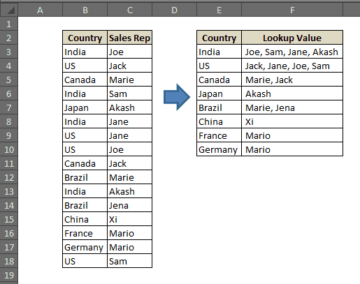
Below I have a data set where I have the names of the people in column A and the training that they have taken in column B.
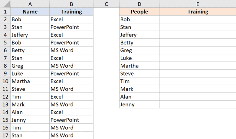
Click here to download the example file and follow along
For each person, I want to find out what training they have completed. In column D, I have the list of unique names (from column A), and I want to quickly lookup and extract all the training that every person has done and get these in a single set (separated by a comma).
Below is the formula that will do this:
=TEXTJOIN(", ",TRUE,IF(D2=$A$2:$A$20,$B$2:$B$20,""))
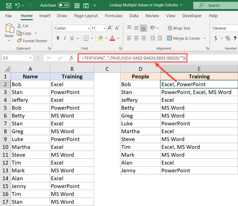
After entering the formula in cell E2, copy it for all the cells where you want the results.
How does this formula work?
Let me deconstruct this formula and explain each part in how it comes together gives us the result.
The logical test in the IF formula (D2=$A$2:$A$20) checks whether the name cell D2 is the same as that in range A2:A20.
It goes through each cell in the range A2:A20, and checks whether the name is the same in cell D2 or not. if it’s the same name, it returns TRUE, else it returns FALSE.
So this part of the formula will give you an array as shown below:
{TRUE;FALSE;FALSE;TRUE;FALSE;FALSE;FALSE;FALSE;FALSE;FALSE;FALSE;FALSE;FALSE;FALSE;FALSE;FALSE;FALSE;FALSE;FALSE}
Since we only want to get the training for Bob (the value in cell D2), we need to get all the corresponding training for the cells that are returning TRUE in the above array.
This is easily done by specifying [value_if_true] part of the IF formula as the range that has the training. This makes sure that if the name in cell D2 matches the name in the range A2:A20, the IF formula would return all the training that person has taken.
And wherever the array returns a FALSE, we have specified the [value_if_false] value as “” (blank), so it returns a blank.
The IF part of the formula returns the array as shown below:
{“Excel”;””;””;”PowerPoint”;””;””;””;””;””;””;””;””;””;””;””;””;””;””;””}
Where it has the names of the training Bob has taken and blanks wherever the name was not Bob.
Now, all we need to do is combine these training name (separated by a comma) and return it in one cell.
And that can easily be done using the new TEXTJOIN formula (available in Excel 2019 and Excel in Microsoft 365)
The TEXTJOIN formula takes three arguments:
- the Delimiter – which is “, ” in our example, as I want the training to separated by a comma and a space character
- TRUE – which tells the TEXTJOIN formula to ignore empty cells and only combine ones that are not empty
- The If formula that returns the text that needs to be combined
If you’re using Excel in Microsoft 365 that already has dynamic arrays, you can just enter the above formula and hit enter. And if you’re using Excel 2019, you need to enter the formula, and hold the Control and the Shift key and then press Enter
Click here to download the example file and follow along
Get Multiple Lookup Values in a Single Cell (without repetition)
Since the UNIQUE formula is only available fro Excel in Microsoft 365, you won’t be able to use this method in Excel 2019
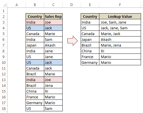
In case there are repetitions in your data set, as shown below, you need to change the formula a little bit so that you only get a list of unique values in a single cell.
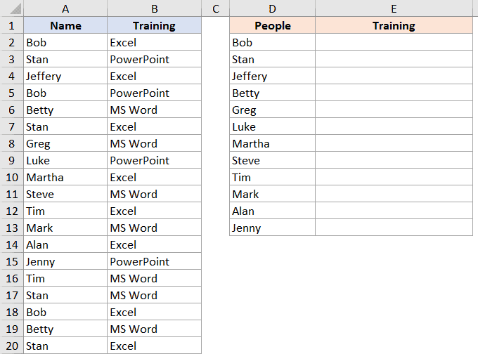
In the above data set, some people have taken training multiple times. For example, Bob and Stan have taken the Excel training twice, and Betty has taken MS Word training twice. But in our result, we do not want to have a training name repeat.
You can use the below formula to do this:
=TEXTJOIN(", ",TRUE,UNIQUE(IF(D2=$A$2:$A$20,$B$2:$B$20,"")))
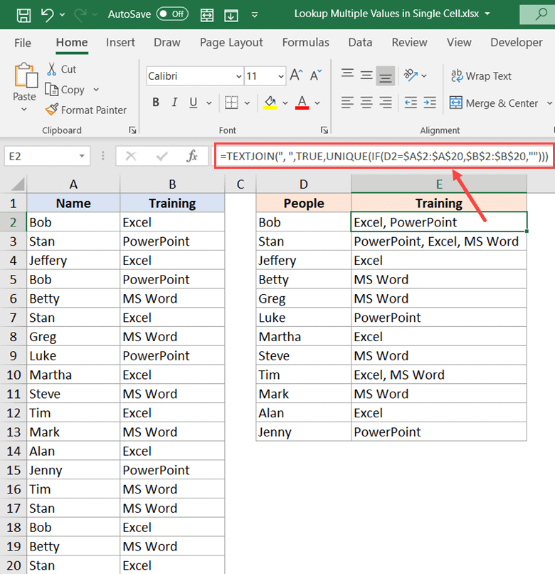
The above formula works the same way, with a minor change. we have used the IF formula within the UNIQUE function so that in case there are repetitions in the if formula result, the UNIQUE function would remove it.
Click here to download the example file
Lookup and Return Multiple Values in One Cell (Using VBA)
If you’re using Excel 2016 or prior versions, then you will not have access to the TEXTJOIN formula. So the best way to then look up and get multiple matching values in a single cell is by using a custom formula that you can create using VBA.
To get multiple lookup values in a single cell, we need to create a function in VBA (similar to the VLOOKUP function) that checks each cell in a column and if the lookup value is found, adds it to the result.
Here is the VBA code that can do this:
'Code by Sumit Bansal (https://trumpexcel.com)
Function SingleCellExtract(Lookupvalue As String, LookupRange As Range, ColumnNumber As Integer)
  Dim i As Long
  Dim Result As String
  For i = 1 To LookupRange.Columns(1).Cells.Count
  If LookupRange.Cells(i, 1) = Lookupvalue Then
  Result = Result & " " & LookupRange.Cells(i, ColumnNumber) & ","
  End If
  Next i
  SingleCellExtract = Left(Result, Len(Result) – 1)
  End Function
Where to Put this Code?
- Open a workbook and click Alt + F11 (this opens the VBA Editor window).
- In this VBA Editor window, on the left, there is a project explorer (where all the workbooks and worksheets are listed). Right-click on any object in the workbook where you want this code to work, and go to Insert –> Module.
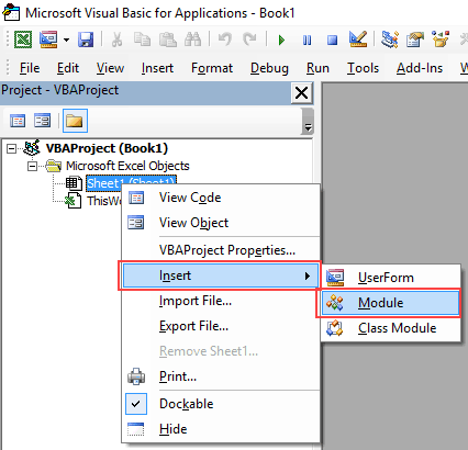
- In the module window (that will appear on the right), copy and paste the above code.
- Now you are all set. Go to any cell in the workbook and type =SingleCellExtract and plug in the required input arguments (i.e., LookupValue, LookupRange, ColumnNumber).
How does this formula work?
This function works similarly to the VLOOKUP function.
It takes 3 arguments as inputs:
1. Lookupvalue – A string that we need to look-up in a range of cells.
2. LookupRange – An array of cells from where we need to fetch the data ($B3:$C18 in this case).
3. ColumnNumber – It is the column number of the table/array from which the matching value is to be returned (2 in this case).
When you use this formula, it checks each cell in the leftmost column in the lookup range and when it finds a match, it adds to the result in the cell in which you have used the formula.
Remember: Save the workbook as a macro-enabled workbook (.xlsm or .xls) to reuse this formula again. Also, this function would be available only in this workbook and not in all workbooks.
Click here to download the example file
Learn how to automate boring repetitive tasks with VBA in Excel. Check out this Free VBA Course
Get Multiple Lookup Values in a Single Cell (without repetition)
There is a possibility that you may have repetitions in the data.
If you use the code used above, it will give you repetitions in the result as well.
If you want to get the result where there are no repetitions, you need to modify the code a bit.
Here is the VBA code that will give you multiple lookup values in a single cell without any repetitions.
'Code by Sumit Bansal (https://trumpexcel.com)
Function MultipleLookupNoRept(Lookupvalue As String, LookupRange As Range, ColumnNumber As Integer)
Dim i As Long
Dim Result As String
For i = 1 To LookupRange.Columns(1).Cells.Count
  If LookupRange.Cells(i, 1) = Lookupvalue Then
    For J = 1 To i - 1
    If LookupRange.Cells(J, 1) = Lookupvalue Then
      If LookupRange.Cells(J, ColumnNumber) = LookupRange.Cells(i, ColumnNumber) Then
        GoTo Skip
      End If
    End If
    Next J
    Result = Result & " " & LookupRange.Cells(i, ColumnNumber) & ","
Skip:
  End If
Next i
MultipleLookupNoRept = Left(Result, Len(Result) - 1)
End FunctionOnce you have placed this code in the VB Editor (as shown above in the tutorial), you will be able to use the MultipleLookupNoRept function.
Here is a snapshot of the result you will get with this MultipleLookupNoRept function.
Click here to download the example file
In this tutorial, I covered how to use formulas and VBA in Excel to find and return multiple lookup values in one cell in Excel.
While it can easily be done with a simple formula if you’re using Excel in Microsoft 365 subscription, if you’re using prior versions and don’t have access to functions such as TEXTJOIN, you can still do this using VBA by creating your own custom function.
You May Also Like the Following Excel Tutorials:


How can I sort or filter with multiple text in a cell (vijay ajay maruti ravi john), I am looking for a solution filter with condition of ajay ravi john. Can you please help me with this?
Thank you
for some reason when i put the VBA code in and go to run it it keeps coming up with an error on this section – Function SingleCellExtract(Lookupvalue As String, LookupRange As Range, ColumnNumber As Integer) and i’m not sure why can you help?
how can i lookup multiple values in a single cell separated by symbol
list1
OP512E08,OP513N16
OP435R74,OP647C84,OP747B38
OP12F45,OP832J43,OP21P67,OP495G74
list2
PRODUCT55,OP513N16,PROODUCT61,OP495G74 ——————————————> 1
OP512E08,PRODUCT31,PRODUCT48,PRODUCT19,OP513N16 ————————> 2
PRODUCT43,OP495G74,PRODUCT22,OP747B38,PRODUCT74,PRODUCT23—–> 3
EXPECTED RESULTS
2,1,2
3
1,3
i ’d like lookup about all parts of list1 in all list2 but results of every cell be in one cell as the expected results
thank u
I want to limit the number of multiple values in excel dropdown
Hi,
Thanks a lot for this awesome code to fetch multiple values in a single cell and without repetition. It worked perfectly for me.
The only problem is that it runs only once till file is opened. The moment I reopen the file and recalculate the formula, it stops working and doesn’t resume even after pasting the code again. I also saved the file as “Macro-enabled” file but it still didn’t solve the issue.
Any help on this problem?
Thanks a lot.
When 2 Criteria Match then Return Multiple Lookup Values In One Comma Separated Cell
A2=B2 Then Result From Range by “fLookUpMultiple” – Please…….
Great code, first one didn’t work for me, but second one that ensures there are not multiple values in the results, works great! Thank you!
Hi,
I’m wanting to get values from multiple items selected from a drop down list (which are listed in the same cell, each on a new line) and have the values of each, listed in the next cell, each on a new line.
Is this possible?
Can I send you my current file, so you can see what I’m working with?
thanks
Hi,
Thanks a lot for this solution.
But would there be an option that it checks each cell in (not only column A) lets say the A+B+C column and that it will return me the value of column D?
Thanks,
Hi,
I tried to use this formula and it works great.
But i have a question:
Would it be possible that not only the values from collum C will be returned but also of for example values from Collum D and E?
Thanks for your help,
I am trying to run this against the email Addresses however I am not getting the results as mentioned. Please help I have already exhausted everything I can. I have saved exactly as mentioned in the document however the output gives me #Value Error
Anyway to get the results to sum. I.e. If the results are values, say 10.3, 5.1, 7.5, I want it to return the sum of these values, so 22.9
How do I do it across 2 different workbooks? Need to lookup a value (input by user in a cell) — compare it in another workbook and respond back with a corresponding number(s) associated against it (2 columns to the left) — output all in 1 cell separated and not duplicated. Thanks
There are only two column but I have 3 Columns then how to do?
Hi Sumit Sir, I receive your excel mail subscription and i visit your website is really deep knowledge and concept clearing. And this code Function MultipleLookupNoRept is really awesome.
Heartily Thanks…
Hello,I want to know if it is possible to nest the MultipleLookupNoRept function as it will not work with the IF functions I have been trying to use it with. Thanks.
hi can someone help me for the singlecellextract is it possible to use this udf if my lookupvalue is a comma separated value?
Hi,
I am very new to VBA, i have a scenario as below.
1. Connect to DB,
2. Execute the query (result will be a single column value)
3. Store the query result into a single cell as List value.
Can anyone please help me getting this work. Thanks!!!
This works great but I think I may have run into a limitation that it will not look at more that about 91,000 rows to match against. I have about 800,000 rows that I need this to look through
How to dropdown list with in multiple lookup cell
Hello Sumit,
Your VBA code is fantastic and its serving my purpose to a great extent.
But i am facing another problem which needs to solved. Please help me with the coding.
Problem is in the desired ColumnNumberi.e result column some cells are blank. So your code is accepting the blank value(with a delimiter) along with other values.
Below example will clear the problem:
Col A Col B Col C Col D
(Sales Person) ( Products) (Sales Pearson) (Result)
1 Superman Toy Superman Toy, , Staionery
2 Spiderman Spiderman , , Toy
3 Batman Stationery Batman Stationery, Toy, Soap
4 Krishh Grocery Krishh Grocery, ,Soap
5 Superman
6 Spiderman Grocery
7 Batman Toy
8 Krishh
9 Superman Stationery
10 Spiderman Toy
11 Batman Soap
12 Krishh Soap
Would anyone help me with macro for a shift schedule of operators working in 2 shifts.
It should choose operators from database and populate in the shift tables according to their expertise in relevant machine?
excellent
How do i get this to work as a Hlookup?
Hi there. I want to do something similar to this. I have a table with people named in row 2, and the date all the way down column 2. I want to be able to generate a comma separated list of those who are on annual leave “AL” for each corresponding day.
Something like this:
date P1 P2 P3 AL
1/1 AL
2/1 AL AL AL P1,P2, P3
3/1 AL AL P1,P2
So it’s similar to your code, but looks along a row, instead of down a column.
Thanks
Hi Craig,
You could do this with a bunch of if statements in the final column. =If (B2=”AL”,$B$1,””) & If (C2=”AL”,” “&$C$1,””) etc. Won’t be comma separated though. Written on phone so excuse mistakes.
I need to use this code on a different worksheet – from the one the list is created on. What do I need to edit to make that happen? Not much of a coder at all….
Same issue for me. I need this to work on another worksheet. Were you able to figure it out?
Hello Sumit,
I found your Multiple lookup values in one ell in your forum and it helped me a lot.
Now i need to improve that and I need your help regarding this.
We have used a code for only one column or a cell as a lookup reference. Now I need to include one more to this. 2 columns as s lookup reference to get the same results.
My code as per your example code is below.
Function SingleCellExtractInward(lookupvalue As String, lookuprange As Range, ColumnNumber As Integer)
Dim i As Double
Dim Result1 As String
Dim Result2 As String
If Result2 = Empty Then
Result2 = “no recent inward”
SingleCellExtractInward = Result2
End If
For i = 1 To lookuprange.Columns(1).Cells.Count
If lookuprange.Cells(i, 1) = lookupvalue Then
Result1 = Result1 & ” ” & lookuprange.Cells(i, ColumnNumber) & “,”
SingleCellExtractInward = Left(Result1, Len(Result1) – 1)
End If
Next i
End Function
Could you please help me on this code to lookup 2 columns as a reference.?
Hello, I have found your code and it helped. I have a query that, I need to lookup one more column with the same process. How can i do that? Please help me on this.
Dear Sumit,
It seems it is the thing i am looking for, but it doesn’t work! I get a #Name error. I have put it in the VB editor and saved it as .xslm. First used the function across sheets and doubted this was the problem. Then tried it i a single sheet with an example wit still got the #Name error.
Any idea what i could be doing wrong? Saved it the wrong way or something?
This is fantastic! Is there a simple way to extend this to search through multiple columns, for example, if column D was another list of names (sales rep 2)?
Also, is there a way to exclude blank cells?,If there happened to be a missing name, for example?
Thank you for this. I had found something similar a while back called vlookupall that gives similar results but was a little harder to follow the internal logic.
Hi, I appreciate your post showing how to do this using VBA, however I am wondering if there is a way to do this using only excel formulas?
Hi Sumit,
Your macro does exactly what I require so I am pleased to find it but I cannot get it to work – I am new to VBA so could be just me 🙂
I have included it into my macro enabled spreadsheet and everytime it executes there is a compile error, like the one mentioned by Laura below.
Compile Error:
Syntax Error
SingleCellExtract = Left(Result, (Len(Result) – 1))
I have tried altering the brackets but no improvement. It looks like it cannot find the added function but I am just guessing. Any suggestions?
Could it be a setting local to me on
FIXED!
I think the example xlsm down load is fine but the above code text included some funny error in the call to
SingleCellExtract = Left(Result, Len(Result) – 1)
It seems there is a funny character in there after copy / paste. As I just deleted it and typed it by hand and then it was fine.
Really pleased as does exactly what I need.
hi! thanks for this vba – how do i correct it so the vlookup value is not case sensitive? currently if I’m looking up “Apple” for example, I need to type “Apple”. If I use a lowercase “a”, it doesn’t lookup the value. Thank you!
Hey Ashley.. You can use the following code for it:
Function SingleCellExtract(Lookupvalue As String, LookupRange As Range, ColumnNumber As Integer)
Dim i As Long
Dim Result As String
For i = 1 To LookupRange.Columns(1).Cells.Count
If LCase(LookupRange.Cells(i, 1)) = LCase(Lookupvalue) Then
Result = Result & ” ” & LookupRange.Cells(i, ColumnNumber) & “,”
End If
Next i
SingleCellExtract = Left(Result, Len(Result) – 1)
End Function
THANK YOU SO MUCH!!! it works!!
Hi Sumit, Great Job i was searching for this exact one. i am not getting the value with the cell having particular sting. Kindly help how we can get the cell having particular sting. pls help
for example:
https://uploads.disquscdn.com/images/72b430f0123fb5f1ca1275477c73ded853c901e314ec1f7da59821b316c02e9d.jpg
hI SUMIT,
Can we get code to reverse this function i have multiple HCodes like H310, H302, etc in one column & corrosponding statement in another column like corrosive for these two codes can i get a code to do v lookup for different h code in same cell saperated by coma to their corrosponding statement without repetation for example if two h codes having same statement i get on statement
Lokesh
please sir upload it again ASAP because i need it
Hey.. Sorry for the misisng file.. I have uploaded it!
please sir upload excel file regarding this topic because this excel sheet not found
I wonder if anyone will still respond to this thread….
I am trying to use this macro, but I get the below error:
Compile Error:
Syntax Error
and it highlights the below portion, as the step it get stuck on
SingleCellExtract = Left(Result, Len(Result) – 1)
My data is 3 columns, my formula goes as follows:
=SingleCellExtract(E3,$A:$C,3)
E3 is the value (a number) i want it to find in the range
$A:$C is the range
3 is the 3rd column where i want the formula to look to pull out the results (result is text).
What am i doing incorrectly?
Hello Laura.. Would be great if you could share the file with me. You can send it at sumitbansal@trumpexcel.com
Actually, I have the same problem, even copying your cells to my workbook. How did you resolved it?
Cheers,
Pier
I’m not sure if anyone is still checking this thread, but by trial and error I was able to make it work by adding some additional parentheses around the Len function:
SingleCellExtract = Left(Result, (Len(Result) – 1))
Not sure why VBA prefers it that way now, but it appears to work.
This worked perfectly! Thank you for the tip!
It wasn’t an extra closing parens. The “minus” char, here, is the wrong character. If you copy and paste from this blog, it’s actually the en-dash character. Simply replace it with the minus char.
Hi Sumit,
Another great idea from you. Code optimised and options integrated
Public Function fLookUpMultiple(ByRef LookUpValue As String, _
ByRef LookUpRange As Excel.Range, _
ByRef ColumnNumber As Long, _
Optional ByRef bUnique As Boolean = True) As String ‘Variant
‘Get all values from a list that match specific value
Dim lgRow As Long
Dim strFilter As String
Dim lgElement As Long
For lgRow = 1 To LookUpRange.Columns(1).Cells.Count
If bUnique Then
If LookUpRange.Cells(lgRow, 1).Value2 = LookUpValue Then
For lgElement = 1 To lgRow – 1
If LookUpRange.Cells(lgElement, 1).Value2 = LookUpValue Then
If LookUpRange.Cells(lgElement, ColumnNumber).Value2 = LookUpRange.Cells(lgRow, ColumnNumber).Value2 Then GoTo Skip
End If
Next lgElement
strFilter = strFilter & ” ” & LookUpRange.Cells(lgRow, ColumnNumber) & “,”
Skip:
End If
Else
If LookUpRange.Cells(lgRow, 1).Value2 = LookUpValue Then strFilter = strFilter & ” ” & LookUpRange.Cells(lgRow, ColumnNumber).Value2 & “,”
End If
Next lgRow
‘Delete last “,”
fLookUpMultiple = VBA.Left(strFilter, VBA.Len(strFilter) – 1)
End Function
I have a question! Student names with ID’s and Class groups. How to take the list and use a combo box – select the class and the names appear on another sheet with their ID’s and class name.
Hi Joe.. Have a look at this – http://trumpexcel.com/2013/07/extract-data-from-drop-down-list/
It does what you are looking for, and uses a data validation drop down instead of a combo box. But it can be easily replicated for a combo box as well. Hope this helps!
Great Job Bro…But how can we get the results without duplicates?
Hi Saji, Glad you liked it.
To get values without duplicates, use this code:
Function SingleCellExtract(Lookupvalue As String, LookupRange As Range, ColumnNumber As Integer)
Dim i As Long
Dim Result As String
For i = 1 To LookupRange.Columns(1).Cells.Count
If LookupRange.Cells(i, 1) = Lookupvalue Then
For J = 1 To i – 1
If LookupRange.Cells(J, 1) = Lookupvalue Then
If LookupRange.Cells(J, ColumnNumber) = LookupRange.Cells(i, ColumnNumber) Then
GoTo Skip
End If
End If
Next J
Result = Result & ” ” & LookupRange.Cells(i, ColumnNumber) & “,”
Skip:
End If
Next i
SingleCellExtract = Left(Result, Len(Result) – 1)
End Function
Can u explain me this VB code?