
Excel XLOOKUP function has finally arrived.
If you have been using VLOOKUP or INDEX/MATCH, I am sure you’ll love the flexibility that the XLOOKUP function provides.
In this tutorial, I will cover everything there is to know about the XLOOKUP function and some examples that will help you know how to best use it.
So let’s get started!
What is XLOOKUP?
XLOOKUP is a new function is Office 365 and is a new and improved version of the VLOOKUP/HLOOKUP function.
It does everything VLOOKUP used to do, and much more.
XLOOKUP is a function that allows you to quickly look for a value in a dataset (vertical or horizontal) and return the corresponding value in some other row/column.
For example, if you’ve got the scores for students in an exam, you can use XLOOKUP to quickly check how much a student has scored using the name of the student.
The power of this function will become even more clear as I deep dive into some XLOOKUP examples later in this tutorial.
But before I get into the examples, there is a big question – how do I get access to XLOOKUP?
How to Get Access to XLOOKUP?
As of now, XLOOKUP is only available for the users of Office 365.
So, if you’re using prior versions of Excel (2010/2013/2016/2019), you won’t be able to use this function.
I am also not sure if this would ever be released for prior versions or not (maybe Microsoft can create an add-in the way they did for Power Query). But as of now, you only get to use it if you’re on Office 365.
Click here to upgrade to Office 365
In case you’re already on Office 365 (Home, Personal, or University edition) and don’t have access to it, you can go to the File tab and then click on Account.
There would be an Office Insider program and you can click and join the Office Insider Program. This will give you access to the XLOOKUP function.

I expect XLOOKUP to be available on all Office 365 versions soon.
Note: XLOOKUP is also available for Office 365 for Mac and Excel for the Web (Excel online)
XLOOKUP Function Syntax
Below is the syntax of the XLOOKUP function:
=XLOOKUP(lookup_value, lookup_array, return_array, [if_not_found], [match_mode], [search_mode])

If you’ve used VLOOKUP, you’ll notice that the syntax is quite similar, with some awesome additional features of course.
Don’t worry if the syntax and argument look a bit too much. I cover these with some easy XLOOKUP examples later in this tutorial that will make it crystal clear.
XLOOKUP function can tale 6 arguments (3 mandatory and 3 optional):
- lookup_value – the value that you’re looking for
- lookup_array – the array in which you’re looking for the lookup value
- return_array – the array from which you want to fetch and return the value (corresponding to the position where the lookup value is found)
- [if_not_found] – the value to return in case the lookup value is not found. In case you don’t specify this argument, a #N/A error would be returned
- [match_mode] – Here you can specify the type of match you want:
- 0 – Exact match, where the lookup_value should exactly match the value in the lookup_array. This is the default option.
- -1 – Looks for the exact match, but if it’s found, returns the next smaller item/value
- 1 – Looks for the exact match, but if it’s found, returns the next larger item/value
- 2 – To do partial matching using wildcards (* or ~)
- [search_mode] – Here you specify how the XLOOKUP function should search the lookup_array
- 1 – This is the default option where the function starts looking for the lookup_value from the top (first item) to the bottom (last item) in the lookup_array
- -1 – Does the search from bottom to top. Useful when you want to find the last matching value in the lookup_array
- 2 – Performs a binary search where the data needs to be sorted in ascending order. If not sorted, this can give error or wrong results
- -2 – Performs a binary search where the data needs to be sorted in descending order. If not sorted, this can give error or wrong results
XLOOKUP Function Examples
Now let’s get to the interesting part – some practical XLOOKUP examples.
These examples will help you better understand how XLOOKUP works, how it’s different from VLOOKUP and INDEX/MATCH and some enhancements and limitations of this function.
Click here to download the example file and follow along
Example 1: Fetch a Lookup Value
Suppose you have the following dataset and you want to fetch the math score for Greg (the lookup value).

Below is the formula that does this:
=XLOOKUP(F2,A2:A15,B2:B15)

In the above formula, I have just used the mandatory arguments where it looks for the name (from top to bottom), finds an exact match, and returns the corresponding value from B2:B15.
One obvious difference the XLOOKUP and VLOOKUP function has is the way they handle lookup array. In VLOOKUP, you have the entire array where the lookup value is in the left-most column and then you specify the column number from where you want to fetch the result. XLOOKUP, on the other hand, allows you to choose lookup_array and return_array separately
One instant benefit of having the lookup_array and return_array as separate arguments means that now you can look to the left. VLOOKUP had this limitation where you can only look up and find a value that is to the right. But with XLOOKUP, that limitation is gone.
Here is an example. I have the same dataset, where the name is on the right and the return_range is on the left.

Below is the formula that I can use to get the score for Greg in Math (which means looking to the left of the lookup_value)
=XLOOKUP(F2,D2:D15,A2:A15)

XLOOKUP solves another major issue – In case you insert a new column, or move columns around, the resulting data would still be correct. VLOOKUP would likely break or give an incorrect result in such cases as most times the column index value is hard-coded.
Example 2: Lookup and Fetch an Entire Record
Let’s take the same data as an example.
In this case, I don’t want to just fetch Greg’s score in Math. I want to get the scores in all the subjects.

In this case, I can use the below formula:
=XLOOKUP(F2,A2:A15,B2:D15)

The above formula uses a return_array range that is more than a column (B2:D15). So when the lookup value is found in A2:A15, the formula returns the entire row from the return_array.
Also, you can not delete just cells that are part of the array that were automatically populated. In this example, you can not delete H2 or I2. If you try, nothing would happen. If you select these cells, the formula in the formula bar would be grayed out (indicating that it can not be changed)
You can delete the formula in cell G2 (where we originally entered it), it will delete the entire result.
This is a useful enhancement as earlier with VLOOKUP, you will have to specify the column number separately for each formula.
Example 3: Two Way Lookup Using XLOOKUP (Horizontal & Vertical Lookup)
Below is a dataset where I want to know the score of Greg in Math (the subject in cell G2).
This can be done using a two-way lookup where I look for the name in column A and the subject name in row 1. The benefit of this two-way lookup is that the result is independent of the student name of the subject name. If I change the subject name to Chemistry, this two-way XLOOKUP formula would still work and give me the correct result.
Below is the formula that will perform the two-way lookup and give the correct result:
=XLOOKUP(G1,B1:D1,XLOOKUP(F2,A2:A15,B2:D15))

This formula uses a Nested XLOOKUP, where first I use it to fetch all the marks of the student in cell F2.
So the result of XLOOKUP(F2,A2:A15,B2:D15) is {21,94,81}, which is an array of marks scored by Greg in this case.
This is then used again within the outer XLOOKUP formula as the return array. In the outer XLOOKUP formula, I look for the subject name (which is in cell G1) and the lookup array is B1:D1.
If the subject name is Math, this outer XLOOKUP formula fetches the first value from the return array – which is {21,94,81} in this example.
This does the same that was, until now, achieved using the INDEX and MATCH combo
Click here to download the example file and follow along
Example 4: When Lookup Value is Not Found (Error Handling)
Error handling has now been added to the XLOOKUP formula.
The fourth argument in the XLOOKUP function is [if_not_found], where you can specify what you want in case the lookup can not be found.
Suppose you have the dataset as shown below where you want to get the Math score in case if the match, and in case the name is not found, you want to return – ‘Did not appear’

The below formula will do this:
=XLOOKUP(F2,A2:A15,B2:B15,"Did not appear")

In this case, I have hard-coded what I want to get in case there is no match. You can also use a cell reference to a cell or a formula.
Example 5: Nested XLOOKUP (Lookup in Multiple Ranges)
The genius of having the [if_not_found] argument is that it allows you to use nested XLOOKUP formula.
For example, suppose you have two separate lists as shown below. While I have these two tables on the same sheet, you can have these in separate sheets or even workbooks.

Below is the nested XLOOKUP formula that will check for the name in both the tables and return the corresponding value from the specified column.
=XLOOKUP(A12,A2:A8,B2:B8,XLOOKUP(A12,F2:F8,G2:G8))

In the above formula, I have used the [if_not_found] argument to use another XLOOKUP formula. This allows you to add the second XLOOKUP in the same formula and scan two tables with a single formula.
I am not sure how many nested XLOOKUPs you can use in a formula. I tried till 10 and it worked, then I gave up 🙂
Example 6: Find the Last Matching Value
This one was badly needed and XLOOKUP made this possible. Now you don’t need to find convoluted ways to get the last matching value in a range.
Suppose you have the dataset as shown below and you want to check when was the last person hired in each department and what was the hire date.

The below formula will lookup the last value for each department and give the name of the last hire:
=XLOOKUP(F1,$B$2:$B$15,$A$2:$A$15,,,-1)
And the below formula will give the hire date of the last hire for each department:
=XLOOKUP(F1,$B$2:$B$15,$C$2:$C$15,,,-1)

Since XLOOKUP has an inbuilt feature to specify the direction of the lookup (first to last or last to first), this is done with a simple formula. With vertical data, VLOOKUP and INDEX/MATCH always look from top to bottom, but with XLOOKUP and can specify the direction as bottom to top as well.
Example 7: Approximate Match with XLOOKUP (Find Tax Rate)
Another notable improvement with XLOOKUP is that now there are four match modes (VLOOKUP has 2 and MATCH has 3).
You can specify any one of the four arguments to decide how the lookup value should be matched:
- 0 – Exact match, where the lookup_value should exactly match the value in the lookup_array. This is the default option.
- -1 – Looks for the exact match, but if it’s found, returns the next smaller item/value
- 1 – Looks for the exact match, but if it’s found, returns the next larger item/value
- 2 – To do partial matching using wildcards (* or ~)
But the best part is that you don’t need to worry whether your data is sorted in an ascending order or descending order. Even if the data is not sorted, XLOOKUP will take care of it.
Below I have a dataset where I want to find the commission of each person – and the commission needs to be calculated using the table on the right.

Below is the formula that will do this:
=XLOOKUP(B2,$E$2:$E$6,$F$2:$F$6,0,-1)*B2

This simply uses the sales value as the lookup and looks through the lookup table on the right. In this formula, I have used -1 as the fifth argument ([match_mode]), which means that it will look for an exact match, and when it doesn’t find one, it will return the value just smaller than the lookup value.
And as I said, you don’t need to worry whether your data is sorted on not.
Click here to download the example file and follow along
Example 8: Horizontal Lookup
XLOOKUP can do vertical as well as a horizontal lookup.
Below I have a dataset where I have student names and their scores in rows, and I want to fetch the score for the name in cell B7.

The below formula will do this:
=XLOOKUP(B7,B1:O1,B2:O2)

This is nothing but a simple lookup (similar to what we saw in Example 1), but horizontal.
All the examples that I cover about vertical lookup can also be done with a horizontal lookup using XLOOKUP (farewell to VLOOKUP and HLOOKUP).
Example 9: Conditional Lookup (Using XLOOKUP with Other Formulas)
This one is a slightly advanced example, and also shows the power of XLOOKUP when you need to do complex lookups.
Below is a data set where I have the names of students and their scores, and I want to know the name of the student who has scored the maximum in each subject and the count of students who has scored more than 80 in each subject.

Below is the formula that will give the name of the student with the highest marks in each subject:
=XLOOKUP(MAX(XLOOKUP(G1,$B$1:$D$1,$B$2:$D$15)),XLOOKUP(G1,$B$1:$D$1,$B$2:$D$15),$A$2:$A$15)
Since XLOOKUP can be used to return an entire array, I have used it to first get all the marks for the required subject.
For example, for Math, when I use XLOOKUP(G1,$B$1:$D$1,$B$2:$D$15), it gives me all the scores in math. I can then use the MAX function to find the maximum score in this range.
This maximum score then becomes my lookup value, and the lookup range would be the array returned by XLOOKUP(G1,$B$1:$D$1,$B$2:$D$15)
I use this within another XLOOKUP formula to fetch the name of the student who has scored the maximum marks.
And to count the number of students who have scored more than 80, use the below formula:
=COUNTIF(XLOOKUP(G1,$B$1:$D$1,$B$2:$D$15),">80")
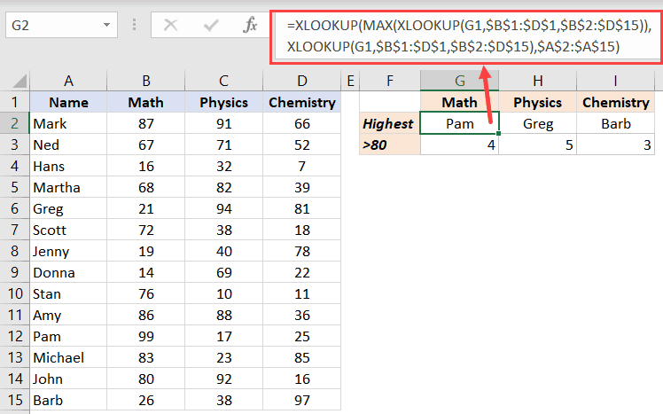
This one simply uses the XLOOKUP formula to get a range of all the values for the given subject. It then wraps it in COUNTIF function to get the number of scores that are more than 80.
Example 10: Using Wildcard in XLOOKUP
Just like you can use wildcard characters in VLOOKUP and MATCH, you can also do this with XLOOKUP.
But there is a difference.
In XLOOKUP, you need to specify that you’re using wildcard characters (in the fifth argument). If you don’t specify this, XLOOKUP will give you an error.
Below is a dataset where I have company names and their market capitalization.

I want to look up a company name in column D, and fetch the market capitalization from the table on the left. And since the names in Column D are not exact matches, I will have to use wildcard characters.
Below is the formula that will do this:
=XLOOKUP("*"&D2&"*",$A$2:$A$11,$B$2:$B$11,,2)

In the above formula, I have used asterisk (*) wildcard character before as after D2 (it needs to be within double quotes and joined with D2 using ampersand).
This tells the formula to look through all the cells, and if it contains the word in cell D2 (which is Apple), consider it an exact match. No matter how many and what characters are before and after the text in cell D2.
And to make sure XLOOKUP accepts wildcard characters, the fifth argument has been set to 2 (wildcard character match).
Example 11: Find the Last Value in the Column
Since XLOOKUP allows you to search from bottom to top, you can easily find the last value in a list, as well as fetch the corresponding value from a column.
Suppose you have a dataset as shown below and you want to know what’s the last company and what’s the market capitalization of this last company.

The below formula will give you the name of the last company:
=XLOOKUP("*",A2:A11,A2:A11,,2,-1)
And the below formula will give the market cap of the last company in the list:
=XLOOKUP("*",A2:A11,B2:B11,,2,-1)

These formulas again use wildcard characters. In these, I have used asterisk (*) as the lookup value, which means that this would consider the first cell it encounters as an exact match (as asterisk could be any character and any number of characters).
And since the direction is from bottom to top (for the vertically arranged data), it will return the last value in the list.
And the second formula since uses a separate return_range to get the market cap of the last name in the list.
Click here to download the example file and follow along
What if You don’t have XLOOKUP?
Since XLOOKUP will likely only be available to Office 365 users, one way to get it is to upgrade to Office 365.
If you already have Office 365 Home, Personal, or University edition, you already have access to XLOOKUP. All you need to do is join the Office Insider program.
To do this, go to the File tab, click on Account and then click on the Office insider option. There would be an option to join the insider program.
In case you have other Office 365 subscriptions (such as Enterprise), I am sure XLOOKUP and other awesome features (such as dynamic arrays, formulas such as SORT and FILTER) would become available soon.
In case you’re using Excel 2010/2013/2016/2019, you won’t have XLOOKUP, and you will have to continue to use VLOOKUP, HLOOKUP, and INDEX/MATCH combo to get the best out of lookup formulas.
XLOOKUP Backward Compatibility
This is one thing you need to be careful about – XLOOKUP is NOT backward compatible.
This means that if you create a file and use the XLOOKUP formula, and then open it in a version that doesn’t have XLOOKUP, it will show errors.
Since XLOOKUP is a huge step forward in the right direction, I believe this will become the default lookup formula, but it will surely take a few years before getting widely adopted. After all, I still see some people using Excel 2003.
So these are 11 XLOOKUP Examples that can help you do all the lookup and reference stuff done faster and also make it easy to use.
Hope you found this tutorial useful!
You may also like the following Excel tutorials:


Hello Sumit,
I want to do a total of “Physics, Chemistry, Math” in a cell. How can we do that using xlookup?
I tried doing it by using “*” but it’s bringing values from the first column out of three columns. I used this formula : =SUM(XLOOKUP(G4,B4:B15,XLOOKUP(“*”,C3:E3,C4:E15,,2)))
The above formula is spilling range from C4 to C15 but I’m expecting something like “C4 to E4” based on G4 lookup.
Pls help
Deep
Is there any way to find the codding for new functions so I should be able to make it on older versions
FANTASTIC thankyou I learnt a lot today
sumit, your website is well of knowledge!!
I have one question, when I opened our file in my excel & opening the fuction argument of xlookup in your formula it is giving e name error #Name
& even in my other file the formulae not working pls suggest how to deal with it.
Hi Sumit
Great presentation of xlookup. I tried getting instructions for this from other sources but none came close to you in explaining this in clear and logical format.
Great work!
Thanks for commenting Wilfred… Glad you found this tutorial useful!
Thank you very much
This is great news for data hunter/gatherers. I am embarrassed at how excited I got knowing Xlookup now exists. Thanks for the insight and the examples, really paints a detailed picture on how to take advantage of this new formula. 🙂
I am equally embarrassed 🙂 I subscribed to the O365 home version and got instant access to these new functions/features. It’s been many days, and I am still experimenting with these new functions (all my latest videos and have been about these only).
Dynamic Array really changes the way we work in Excel and makes some of the things that used to take a lot of complex formulas really easy.