How to Compare Two Excel Sheets (for Differences)

Comparing two Excel files (or comparing two sheets in the same file) can be tricky as an Excel workbook only shows one sheet at a time.

This becomes more difficult and error-prone when you have a lot of data that needs to be compared.

Thankfully, there are some cool features in Excel that allow you to open and easily compare two Excel files.

In this Excel tutorial, I will show you multiple ways to compare two different Excel files (or sheets) and check for differences.

You can view them side by side, highlight changed cells, or create a formula report. I’ll also cover XLOOKUP, VBA, Power Query, Spreadsheet Compare, and an online tool.

The method you choose will depend on how your data is structured and what kind of comparison you’re looking for.

Let’s get started!

Compare Two Excel Files Side by Side

If you want to compare two separate Excel files side by side, there is an in-built feature in Excel to do this.

It’s the View Side by Side option.

This is recommended only when you have a small dataset and manually comparing these files is likely to be less time-consuming and error-prone.

If you have a large dataset, I recommend using the conditional formatting method or the formula method covered later in this tutorial.

Let’s see how to use this when you have to compare two separate files.

Suppose you have two files for two different months, Jan and Feb, with item prices. You want to check which values changed between the two price lists.

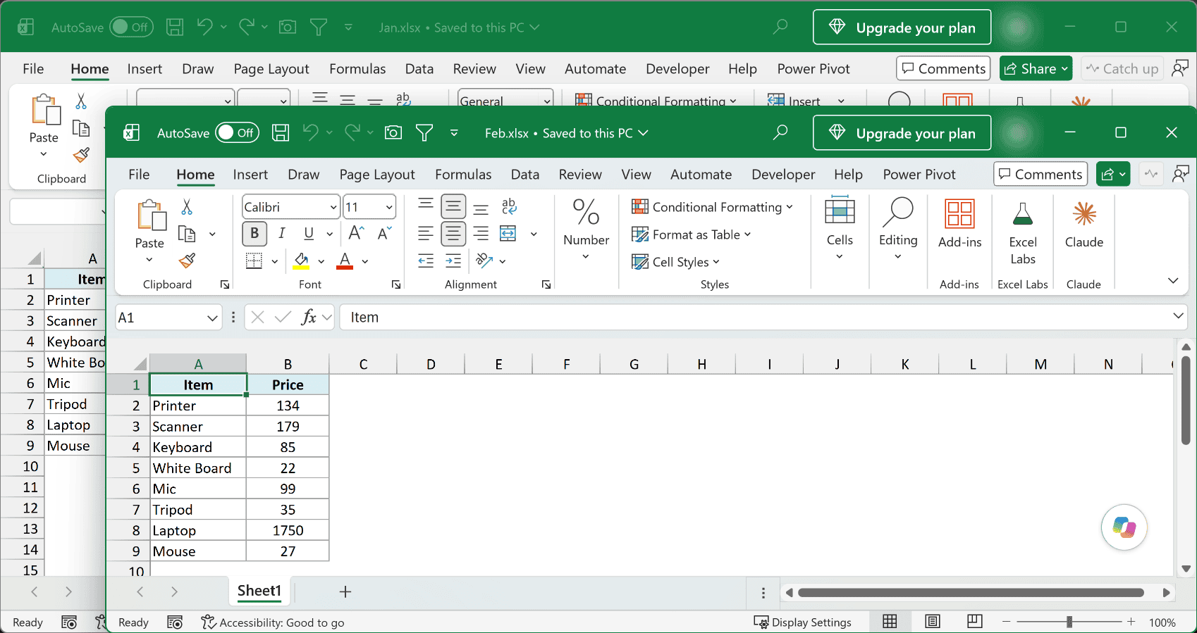
By default, when you open a file, it’s likely to take up your entire screen. Even if you reduce the size, one Excel file stays on top.

View Side by Side lets you arrange both files horizontally or vertically, so you can compare values without switching back and forth.

Below are the steps to align two files side by side and compare them:

1. Open the two Excel files that you want to compare.

2. In the first file, select the sheet that you want to compare.

3. In the second file, select the sheet that you want to compare.

4. Click the View tab.

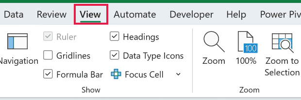
5. In the Window group, click View Side by Side. This becomes available only when you have two or more Excel files open.

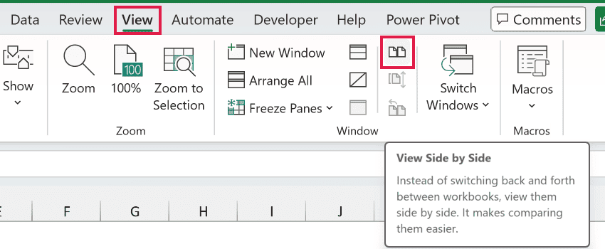
Excel arranges the files horizontally. Both files are visible, and you can edit or compare them while they’re arranged this way.

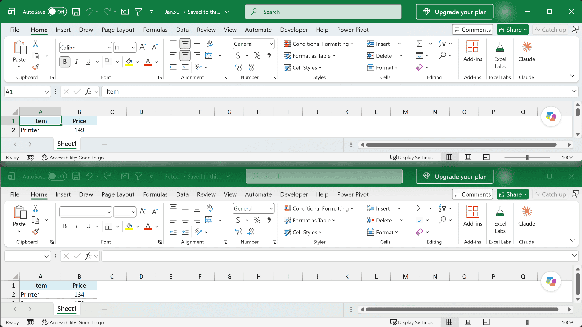
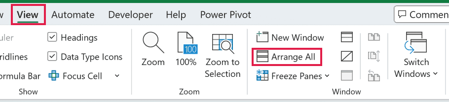
6. To place the files next to each other, click Arrange All (in the View tab).

7. In the Arrange Windows dialog box, select Vertical.

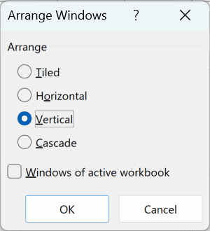
8. Click OK.

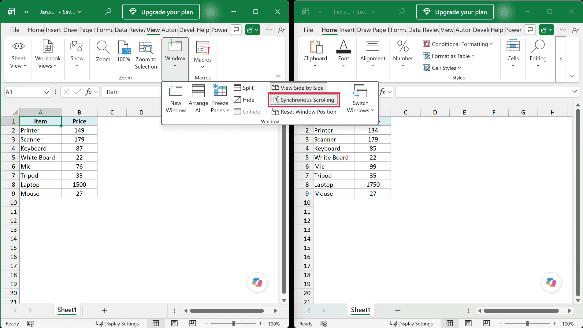
If one sheet scrolls while the other stays still, enable Synchronous Scrolling. This makes it easier to compare the data line by line and spot differences.

Click Synchronous Scrolling in the View tab of either workbook. It’s a toggle button, so clicking it again turns it off.

Comparing Multiple Excel Files Side by Side

With the View Side by Side option, you can only compare two Excel files at one go.

If more than two files are open, clicking View Side by Side opens the Compare Side by Side dialog box. Choose the file to compare with the active workbook.

To see more than two files at once, open all of them and click Arrange All in the View tab.

In the Arrange Windows dialog box, select Vertical or Horizontal, then click OK. Excel arranges all the open files in the selected layout.

If you want to look at two parts of the same sheet, use split screen instead.

Compare Two Sheets in the Same Workbook Using New Window

In case you want to compare two sheets in the same workbook, you can’t start with View Side by Side. You first need a second window for that workbook.

The New Window feature opens a second instance of the same workbook. You can then arrange the windows side by side.

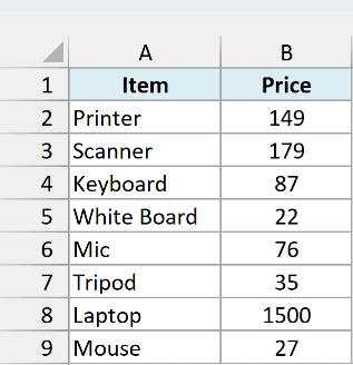
Below I have item prices on the Jan and Feb sheets, and I want to compare them side by side to see which prices changed.

Below are the steps to compare these two sheets in Excel:

1. Open the workbook that contains the Jan and Feb sheets.

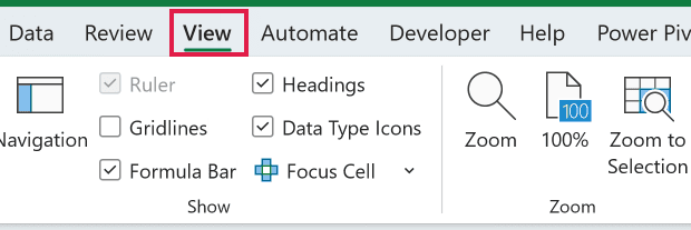
2. Click the View tab.

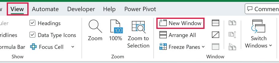
3. In the Window group, click New Window. This opens a second instance of the same workbook.

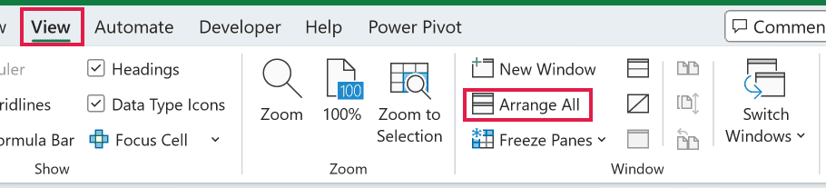
4. In the View tab, click Arrange All to open the Arrange Windows dialog box.

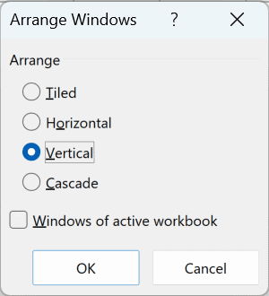
5. Select Vertical to compare data in columns. Select Horizontal if you want to compare data in rows.

If other files are open, also check Windows of active workbook in the Arrange Windows dialog so only this workbook’s two windows are arranged.

6. Click OK.

Both windows now sit next to each other, but they initially show the same worksheet.

7. Select Jan in the left window.

8. Select Feb in the right window so you can compare it with Jan.

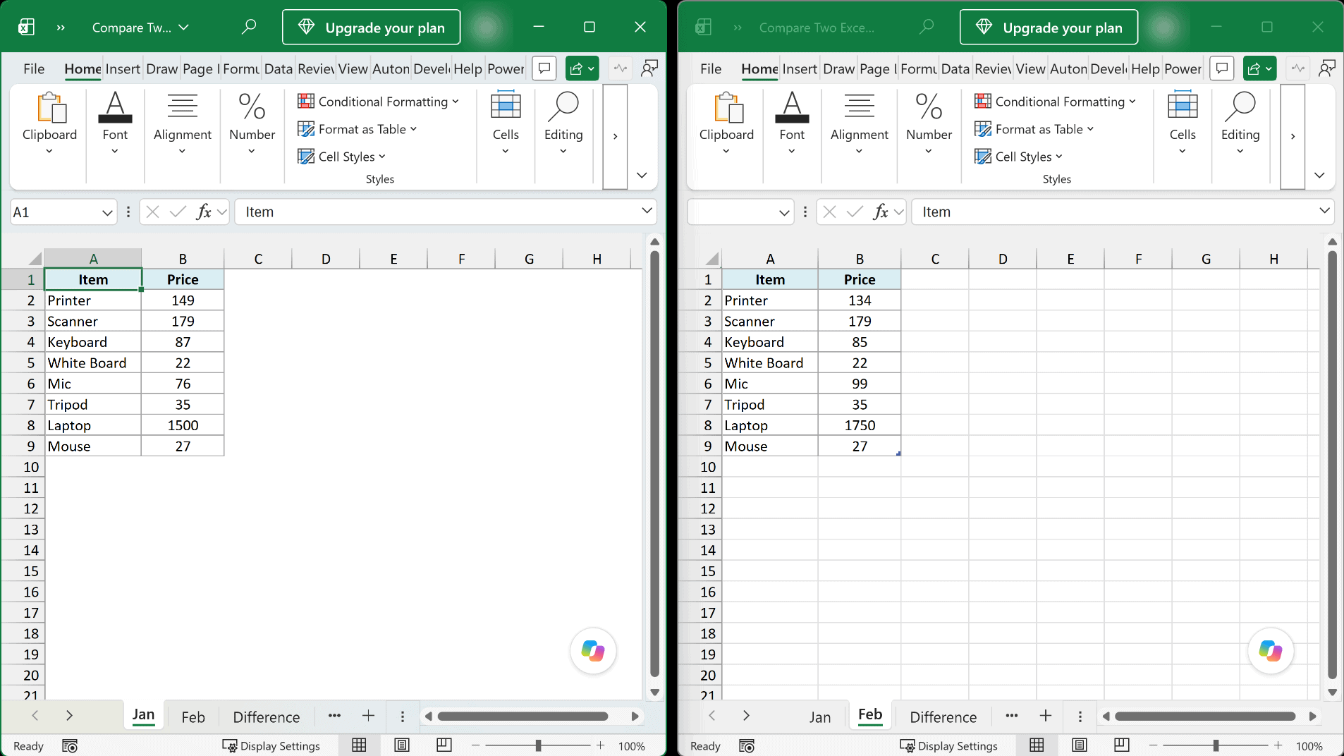
How does this work?

New Window opens another view of the same workbook. The windows get - 1 and - 2 added to the name, for example, Test - 1 and Test - 2.

The title bar may also show the .xlsx extension, depending on your Windows settings.

Note that these are still the same workbook. Any changes you make in either window appear in both.

When you close one of the two windows, the name reverts to the original.

You can also use Synchronous Scrolling here. Enable View Side by Side for the two windows, then click Synchronous Scrolling in the View tab.

Compare Two Sheets and Highlight Differences with Conditional Formatting

Manually comparing data line by line is error-prone when you have a lot of data. Conditional formatting can highlight the differences for you.

This method is really useful if you have two versions in two different sheets and you want to quickly check what has changed.

Conditional formatting can refer to another sheet in the same workbook, but it can’t refer to another workbook.

If your sheets are in separate files, copy the sheet from the other file into the same workbook before creating the rule.

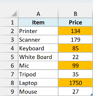
Below I have the same items in the same order on Jan and Feb, and I want to highlight changed prices in Feb’s Price column.

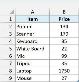
Below are the steps to do this:

1. On the Feb sheet, select B2:B9 (starting from B2), the prices you want to compare.

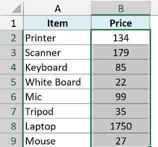
2. Click the Home tab.

3. In the Styles group, click Conditional Formatting.

4. Click New Rule.

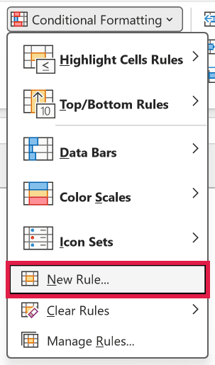
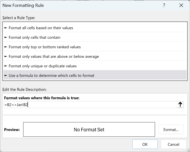
5. In the New Formatting Rule dialog box, select Use a formula to determine which cells to format.

6. In the formula field, enter the formula below.

=B2<>Jan!B2

7. Click Format.

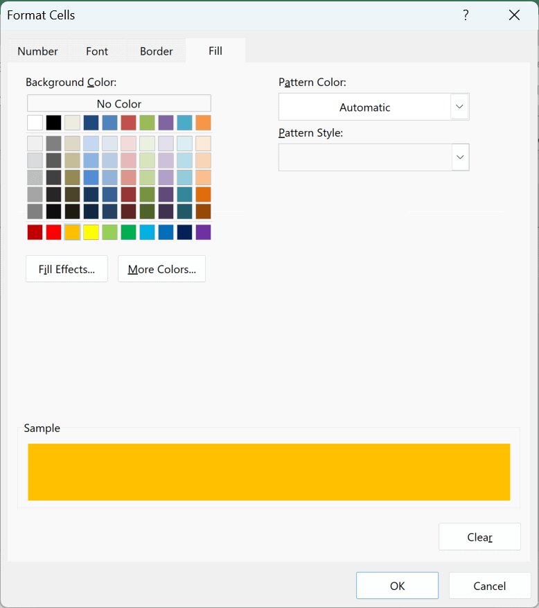
8. In the Format Cells dialog box, click the Fill tab.

9. Select the color you want to use for the changed prices.

10. Click OK to close Format Cells.

11. Click OK to save the rule.

The rule highlights Feb cells B2, B4, B6, and B8. These are Printer (134), Keyboard (85), Mic (99), and Laptop (1750).

How does this work?

Conditional formatting highlights a cell when its rule formula returns TRUE.

The <> operator means “not equal to.” Here, the rule compares Feb!B2 with Jan!B2. If the prices differ, it returns TRUE and highlights the Feb cell.

Note that I have used a relative reference in this example.

It’s B2, not $B$2, $B2, or B$2. As Excel checks each row, the references move together, so the next comparison is Feb!B3 against Jan!B3.

When using this method to compare two sheets in Excel, remember the following:

• It’s useful for a quick check when the rows line up. If you insert a row or delete a row in one sheet, every row below can look different because the items no longer occupy matching cells. It’s not a reliable ongoing comparison if rows keep moving.
• You can only compare sheets in the same Excel file.
• You can compare values only, not differences in formulas or formatting.

Compare Two Sheets and Get the Differences with a Formula

If you want to see both the old and new values for each change, you can use a formula to create a separate difference report.

This method works for two sheets in one workbook or for sheets in two separate workbooks.

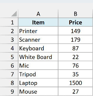
Below I have item prices on the Jan and Feb sheets, and I want to show only the changed values on a separate sheet.

Insert a new worksheet and name it Difference. Type Item in A1 and Price in B1.

In A2, enter the formula below. Select A2:B9 and turn on Wrap Text in the Home tab so the two values display on separate lines.

=IF(Jan!A2:B9<>Feb!A2:B9,"Jan Value: "&Jan!A2:B9&CHAR(10)&"Feb Value: "&Feb!A2:B9,"")

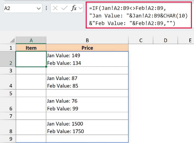
Press Enter once, and the formula spills across A2:B9 on its own. You don’t need to drag it or use Ctrl + Shift + Enter.

This spilling formula works in Excel for Microsoft 365, Excel 2024, Excel 2021, and Excel for the web.

The above formula uses an IF condition to check whether corresponding cells have different values.

If the values match, the IF function returns a blank. If they differ, it returns both values, with Jan Value and Feb Value as labels.

CHAR(10) puts the values on separate lines in the same cell.

You need Wrap Text turned on to see those two lines.

The good thing with this method is that it only gives you the differences and shows you exactly what the difference is.

There are four changed prices in this example:

• B2, Printer: Jan Value: 149 and Feb Value: 134.
• B4, Keyboard: Jan Value: 87 and Feb Value: 85.
• B6, Mic: Jan Value: 76 and Feb Value: 99.
• B8, Laptop: Jan Value: 1500 and Feb Value: 1750.

Every other result cell is blank because its value didn’t change.

The report mirrors the layout of the source sheets, cell for cell. B4 here means cell B4 on both Jan and Feb.

Column A is empty because none of the item names changed. If you renamed an item, its difference would show in column A.

To count the differences, type Total Differences in A11. Enter this formula in B11:

=SUMPRODUCT(--(Jan!A2:B9<>Feb!A2:B9))

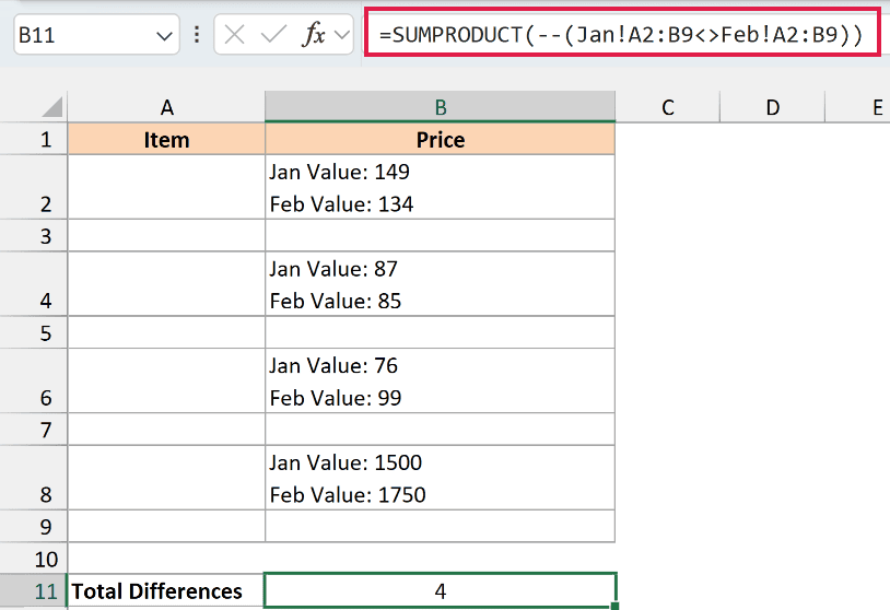
B11 returns 4. The comparison checks which cells have different values, giving TRUE for a difference and FALSE for a match.

The double minus (--) converts TRUE and FALSE to 1 and 0, so the SUMPRODUCT function can add them to count the differences.

This count formula works in every Excel version with a plain Enter. You don’t need Ctrl + Shift + Enter.

Fallback for Excel 2019 and Earlier

In Difference!A2, use the single-cell version below:

=IF(Jan!A2<>Feb!A2,"Jan Value: "&Jan!A2&CHAR(10)&"Feb Value: "&Feb!A2,"")

Copy it across and down to cover A2:B9. Turn on Wrap Text for this range. It gives the same four differences.

Comparing Sheets in Two Separate Files

Keep both files open while setting up the comparison. Replace the sheet references with workbook references, as in this example:

=IF([Jan.xlsx]Sheet1!A2:B9<>[Feb.xlsx]Sheet1!A2:B9,"Jan Value: "&[Jan.xlsx]Sheet1!A2:B9&CHAR(10)&"Feb Value: "&[Feb.xlsx]Sheet1!A2:B9,"")

This compares A2:B9 on Sheet1 in Jan.xlsx with the same range in Feb.xlsx.

To get a reference right, type = and click the cell in the other file. Excel inserts the workbook and sheet name for you.

If you close a source file, Excel switches its reference to the full file path and keeps the existing result.

See how to reference another workbook if your file or sheet names are different.

Match Data in Two Sheets When Rows Are in a Different Order (XLOOKUP)

Conditional formatting and the difference formula compare cells by position. An inserted, deleted, or re-sorted row can break that comparison.

Matching by item solves this. You can find the same item even when it moves to another row.

Below I have the Mar price list, and I want each item’s price from Feb in column C and a Same, Changed, or New label in column D.

The supplier changed the row order in March, added Webcam, and dropped Tripod.

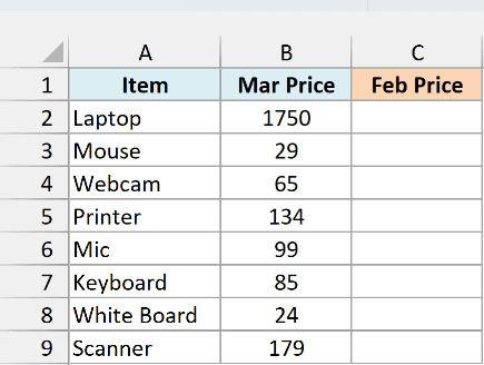
Type Feb Price in C1. In C2, enter this formula:

=XLOOKUP(A2:A9,Feb!A2:A9,Feb!B2:B9,"Not in Feb")

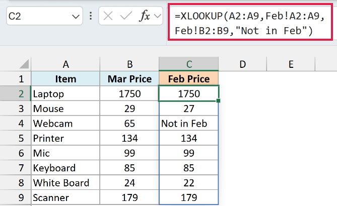
The XLOOKUP function finds each Mar item in Feb’s Item column and returns its price, regardless of row order.

The fourth argument returns Not in Feb when an item has no match. That’s what you see for Webcam.

C2:C9 returns 1750, 27, Not in Feb, 134, 99, 85, 22, and 179, in the order of the March list.

Type Status in D1. In D2, enter this formula:

=IF(C2:C9="Not in Feb","New",IF(B2:B9=C2:C9,"Same","Changed"))

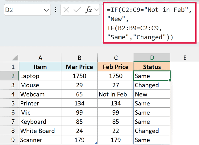
If a March item has no February match, the first IF function labels it New.

Otherwise, the second IF function compares the March and February prices and returns Same or Changed.

D2:D9 returns Same, Changed, New, Same, Same, Same, Changed, and Same.

Mouse changed from 27 to 29, White Board changed from 22 to 24, and Webcam is new. The other March items have the same prices as February.

Both formulas fill their whole result ranges automatically, C2:C9 and D2:D9.

Just press Enter. You don’t need to drag them down or use Ctrl + Shift + Enter.

XLOOKUP and these spilling formulas work in Excel for Microsoft 365, Excel 2024, Excel 2021, and Excel for the web.

This comparison doesn’t show Tripod. It was in Feb but isn’t in Mar, so a lookup starting with March items never looks for it.

To catch removed items, run the lookup the other way.

In an empty column on the Mar sheet (for example, F2), enter:

=XLOOKUP(Feb!A2:A9,A2:A9,B2:B9,"Not in Mar")

These results follow Feb’s item order: 134, 179, 85, 24, 99, Not in Mar, 1750, and 29. Tripod is the item marked Not in Mar.

Or use the Power Query method later in this article to show new and removed items in one table.

Fallback for Excel 2019 and Earlier

In Mar!C2, use this formula and copy it down to C9:

=IFERROR(VLOOKUP(A2,Feb!$A$2:$B$9,2,FALSE),"Not in Feb")

The VLOOKUP function looks for an exact match in the first column of Feb!A2:B9 and returns the price from its second column.

If there is no match, the IFERROR function returns Not in Feb.

This gives the same February prices as the spilling XLOOKUP formula.

If you only need to check which names are missing between two lists, see the comparing two columns tutorial in the related list at the end.

Compare Two Sheets and Highlight Differences Using VBA

If you need to compare Excel files or sheets quite often, it’s a good idea to have a ready Excel macro VBA code and use it whenever you need to make the comparison.

You can also add the macro to the Quick Access Toolbar so that you can run it with a single button and instantly know what cells are different in different files or sheets.

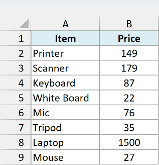
Below I have item prices on the Jan and Feb sheets, and I want to compare them and highlight the differences in Jan.

Here is the VBA code:

Sub CompareSheets()
Dim rngCell As Range

For Each rngCell In Worksheets("Jan").UsedRange

    If CStr(rngCell.Value2) <> CStr(Worksheets("Feb").Cells(rngCell.Row, rngCell.Column).Value2) Then
        rngCell.Interior.Color = vbYellow
    End If

Next rngCell

End Sub

Sub CompareSheets()Dim rngCell As RangeFor Each rngCell In Worksheets("Jan").UsedRange    If CStr(rngCell.Value2) <> CStr(Worksheets("Feb").Cells(rngCell.Row, rngCell.Column).Value2) Then        rngCell.Interior.Color = vbYellow    End IfNext rngCellEnd Sub

It compares both cells as text, so a cell with an error value (like #N/A) doesn’t stop the macro with a Type mismatch error.

Important: The macro changes cell colors in place, and Ctrl + Z can’t undo it. Run it on a copy.

You can use this code in a regular module in the VB Editor. Here are the steps:

1. With the workbook active, press Alt + F11 to open the VB Editor.

2. Click Insert in the VB Editor.

3. Click Module to insert a regular module.

4. Paste the code above into the module.

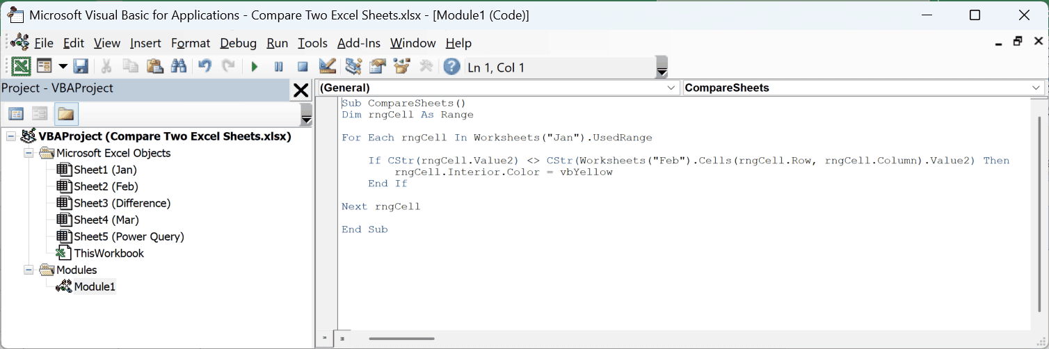
5. With the cursor inside the code, press F5 to run the macro.

The macro highlights Jan cells B2, B4, B6, and B8 in yellow. These are the changed prices for Printer, Keyboard, Mic, and Laptop.

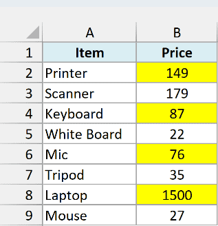
The code uses a For Next loop to check every cell in Jan’s entire used range against the corresponding cell in Feb.

It only checks cells inside Jan’s used range, so a row added at the bottom of Feb won’t be flagged.

The If-Then statement checks for a difference and gives the Jan cell a yellow fill when the values differ.

Save the file as an Excel Macro-Enabled Workbook (.xlsm) if you want to keep the macro in it. The example download is an .xlsx file, so it doesn’t contain the macro.

Comparing Two Open Files

To compare two open files, replace Worksheets("Jan") with Workbooks("Jan.xlsx").Worksheets("Sheet1") in the code.

Then replace Worksheets("Feb") with Workbooks("Feb.xlsx").Worksheets("Sheet1").

Use your actual file and sheet names, and keep both files open.

If you need to do this often, save the code in the Personal Macro Workbook and add it to the Quick Access Toolbar. Then you can run it with a click of a button.

Here are the steps to get the Personal Macro Workbook in Excel.

It’s not available by default, so you need to enable it.

Here are the steps to save this code in the Personal Macro Workbook.

And here you will find the steps to add this macro code to the QAT.

Compare Two Sheets or Files Using Power Query

If you compare price lists every month, Power Query can put changed, new, and removed items into one table. Next month, you just refresh.

You can also compare sheets in two separate files with this method.

Power Query is built into Excel 2016 and later for Windows, and Microsoft 365. You’ll find it in the Data tab’s Get & Transform Data group.

Below I have the Feb and Mar price lists, and I want one report showing changed, new, and removed items.

March has a different row order, a new Webcam, and no Tripod.

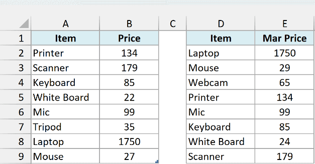
Each list needs to be an Excel Table. Select just the list (A1:B9 here), press Ctrl + T, confirm My table has headers, and click OK. Repeat for the other list.

In Table Design > Table Name, name the tables Feb and Mar. The example file already uses these names.

Feb has Item and Price columns. Mar has Item and Mar Price columns.

Power Query names each source query after its table. Using these names also gives us the expanded columns Mar.Item and Mar.Mar Price later.

If your lists are in separate files, use Data > Get Data > From File > From Excel Workbook for each file, pick its sheet or table in the Navigator, and click Transform Data.

Rename the queries Feb and Mar in the Query Settings pane, then load each as a connection only (Close & Load To > Only Create Connection).

The rest of the steps are the same.

Create a Connection for Each Table

1. Select a cell in the Feb table.

2. Click the Data tab.

3. Click From Table/Range to open the Power Query Editor.

4. In the editor’s Home tab, open the Close & Load drop-down.

5. Click Close & Load To.

6. Select Only Create Connection.

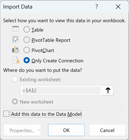
7. Click OK.

8. Repeat steps 1 to 7 for the Mar table to create its connection-only query.

Merge the Two Lists

1. In Excel, click the Data tab.

2. Click Get Data.

3. Choose Combine Queries.

4. Click Merge.

5. In the Merge dialog, select Feb as the top table.

6. Click its Item column.

7. Select Mar as the bottom table.

8. Click its Item column.

9. Set Join Kind to Full Outer (all rows from both).

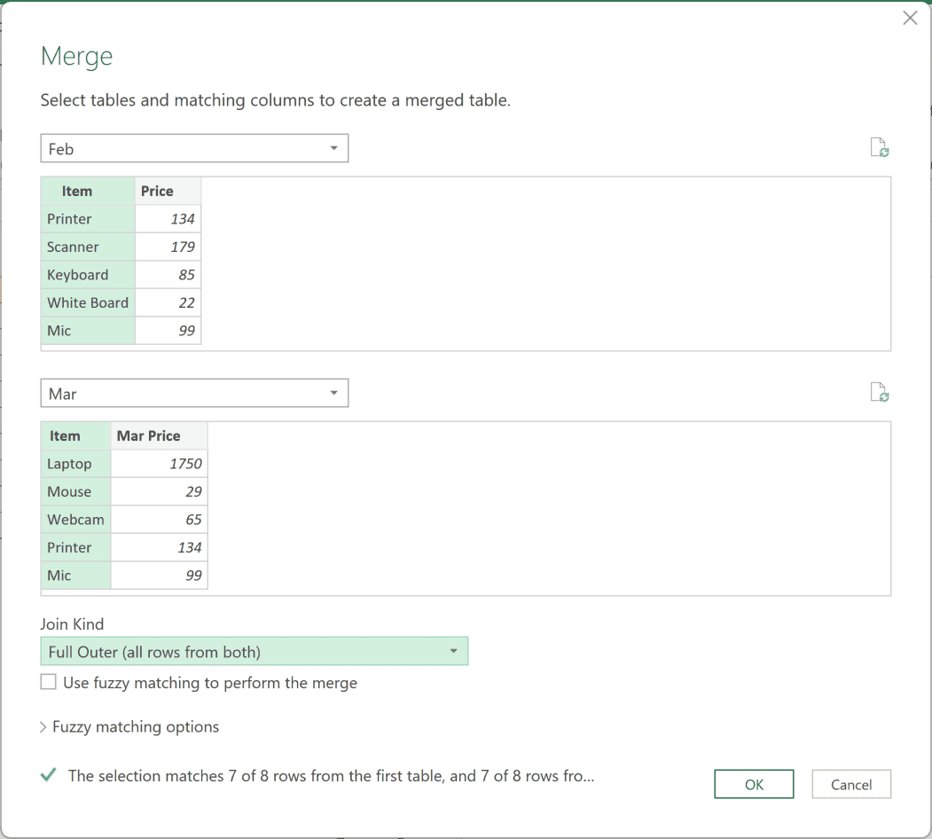
10. Click OK.

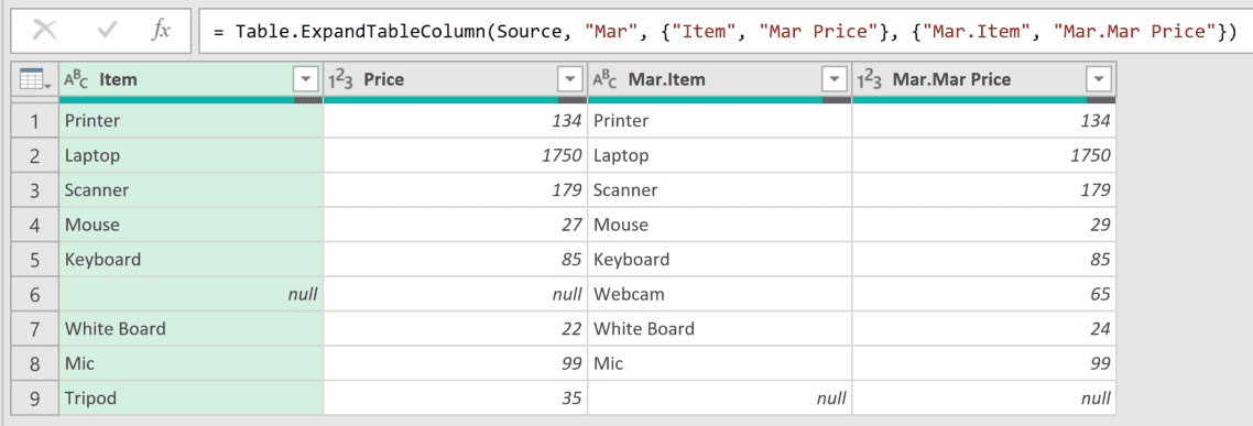
A Full Outer join keeps every item from both lists. This is how Webcam and Tripod make it into the report, even though each is missing from one month.

11. Click the expand icon in the Mar column header.

12. Keep Item and Mar Price checked. Leave Use original column name as prefix on.

13. Click OK.

You now have Mar.Item and Mar.Mar Price beside the February columns.

Fill the Item Name and Add a Status

Webcam has no February match, so its February Item cell is null (Power Query’s marker for a missing value). We’ll fill its name from Mar.Item.

1. In the Add Column tab, click Conditional Column.

2. Name the column Item Name.

3. Set the condition to Item equals null. For the output, choose Select a column and select Mar.Item.

4. For Else, choose Select a column and select Item.

5. Click OK.

6. In the Add Column tab, click Conditional Column again.

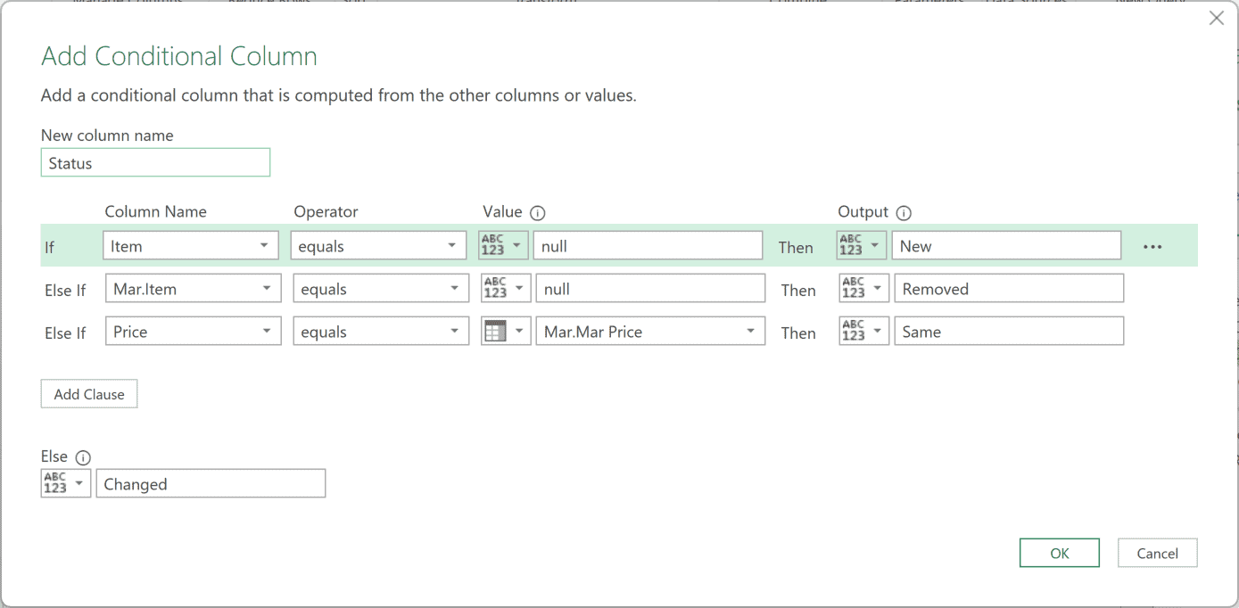
7. Name the column Status.

8. Set the first condition to Item equals null, with New as its output.

9. Add an Else If clause for Mar.Item equals null, with Removed as its output.

10. Add an Else If clause for Price equals the column Mar.Mar Price, with Same as its output. Select a column for the comparison value.

11. Set Else to Changed.

12. Click OK.

These conditions mark items found only in March as New and items found only in February as Removed. For items in both, they compare the two prices.

Finish and Load the Report

1. Remove the Item column.

2. Remove the Mar.Item column.

3. Rename Item Name to Item.

4. Rename Price to Feb Price.

5. Rename Mar.Mar Price to Mar Price.

6. Drag the columns into the order Item, Feb Price, Mar Price, Status.

7. Sort Status ascending.

8. Add Item ascending as the second sort, keeping Status as the first sort.

9. In the Query Settings pane, rename the query Compare.

10. In the Home tab, click Close & Load.

The example file’s Compare query loads the report onto the Power Query sheet in A1:D10. The two changed items appear at the top, followed by New, Removed, and Same.

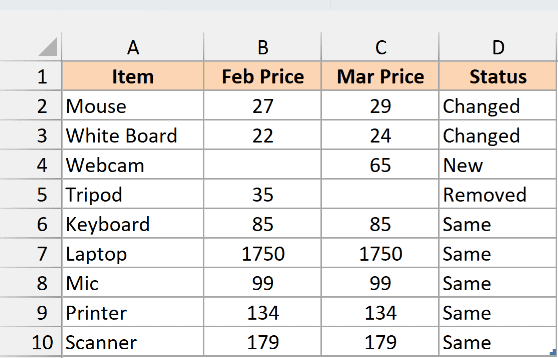
The report contains these rows in this order:

• Mouse: Feb Price 27, Mar Price 29, Changed.
• White Board: Feb Price 22, Mar Price 24, Changed.
• Webcam: Feb Price blank, Mar Price 65, New.
• Tripod: Feb Price 35, Mar Price blank, Removed.
• Keyboard: Feb Price 85, Mar Price 85, Same.
• Laptop: Feb Price 1750, Mar Price 1750, Same.
• Mic: Feb Price 99, Mar Price 99, Same.
• Printer: Feb Price 134, Mar Price 134, Same.
• Scanner: Feb Price 179, Mar Price 179, Same.

Next month, replace the data in the tables (or source files), then click Data > Refresh All. You don’t need to rebuild the comparison.

Power Query treats printer and Printer, or an item with a trailing space, as different items. You could get a Removed row and a New row for the same product.

To fix this, open each source query (Data > Queries & Connections, right-click the query, Edit) and select its Item column.

Use Transform > Format > Trim, then Transform > Format > Capitalize Each Word so the names match.

For more on merging, see Merge Tables in Excel Using Power Query.

Compare Two Excel Files Using Spreadsheet Compare

The methods above compare values. If you also need to check formulas, formatting, or VBA code, Microsoft’s Spreadsheet Compare can compare two workbooks sheet by sheet.

It checks hidden sheets too, and reports changes in entered values, calculated values, formulas, cell formatting, and macros. VBA differences appear side by side.

Spreadsheet Compare is available only in Excel for Windows in Microsoft 365 Apps for enterprise plans and equivalent editions.

It’s also in Office Professional Plus 2013, 2016, and 2019 (and equivalent later volume-licensed editions). It isn’t available on Mac.

Microsoft doesn’t list the Home editions (Microsoft 365 Personal and Family, Office Home) among the editions that include it.

If you don’t see Spreadsheet Compare, your version doesn’t include it. Use one of the other methods in this tutorial.

Here are the steps to compare two files:

1. Open the Windows Start menu.

2. Type Spreadsheet Compare.

3. Open Spreadsheet Compare from the search results.

4. On its Home tab, click Compare Files.

5. Click the folder icon next to Compare and select the older file.

6. Click the folder icon next to To and select the newer file.

7. Click OK.

8. Choose the comparison options, such as Formulas, Macros, Cell Format, or Select All.

9. Click OK to run the comparison.

The files appear in a side-by-side grid, with the older file on the left and the newer file on the right.

A details pane below lists the changes, and a color legend explains the colors. For example, changed entered values get a green fill.

You can also open it through Excel’s Inquire tab > Compare Files with both workbooks open. If the tab isn’t visible, turn on the add-in:

1. Click File.

2. Click Options.

3. Select Add-ins.

4. Set Manage to COM Add-ins.

5. Click Go.

6. Check Inquire.

7. Click OK.

If Inquire isn’t in the list, your version doesn’t include it or your administrator has turned it off.

See Microsoft’s Spreadsheet Compare guide for more details.

Compare Two Excel Files Online Using XL Comparator

Another quick way to compare two Excel files and check for matches and differences is by using a free third-party tool such as XL Comparator.

It’s a web-based tool. You upload two Excel files, and it creates a comparison file containing common or different data, depending on the option you select.

Suppose you have two files with customer names and email addresses. You want to check which customers are in file 1 but aren’t in file 2.

Below is how you compare two Excel files and create a comparison report:

1. Open https://www.xlcomparator.net/.

2. Use Choose file to upload the two files. The maximum size of each file can be 5MB.

3. Click Next.

4. Select the common column in both files. The tool uses this column to look for matches and differences, for example, the customer email address.

5. Select one of the four options: matching data based on File 1, matching data based on File 2, data in File 1 but not File 2, or data in File 2 but not File 1.

6. Click Next.

7. Download the comparison file. It contains the data for the option you selected in step 5.

Below is a video that shows how XL Comparator tool works.

One concern you may have when using a third-party tool to compare Excel files is about privacy.

If you have confidential data and privacy is really important for it, it’s better to use other methods shown above.

The XL Comparator website says it deletes all files 1 hour after you upload them.

If you only need to compare two lists without uploading files, the Compare Two Lists tool runs in your browser and sends nothing to a server.

These are some of the methods you can use to compare two different Excel files (or worksheets in the same Excel file). Hope you found this Excel tutorial useful.

You may also like the following Excel tutorials:

• How to Compare Two Columns in Excel (for matches & differences)
• How to Remove Duplicates in Excel
• How to Compare Text in Excel (Easy Formulas)
• Split Each Excel Sheet Into Separate Files (Step-by-Step)
• Combine Data from Multiple Workbooks in Excel
• Combine Data From Multiple Worksheets into a Single Worksheet in Excel
• How to Compare Dates in Excel (Greater/Less Than, Mismatches)
• How to Enable and Use Track Changes in Excel