
Power Query can be of great help when you want to combine multiple workbooks into one single workbook.
For example, suppose you have the sales data for different regions (East, West, North, and South). You can combine this data from different workbooks into a single worksheet using Power Query.
If you have these workbooks in different locations/folders, it’s a good idea to move all these into a single folder (or create a copy and put that workbook copy in the same folder).
So to begin with, I have four workbooks in a folder (as shown below).

Now, in this tutorial, I am covering three scenarios where you can combine the data from different workbooks using Power Query:
- Each workbook has the data in an Excel Table, and all the table names are same.
- Each workbook has the data with the same worksheet name. This can be the case when there is sheet named ‘summary’ or ‘data’ in all the workbooks, and you want to combine all these.
- Each workbook has many sheets and tables, and you want to combine specific tables/sheets. This method can also be helpful when you want to combine table/sheets that don’t have a consistent name.
Let’s see how to combine data from these workbooks in each case.
Each workbook has the data in an Excel Table with the same structure
The below technique would work when your Excel Tables has been structured the same way (same column names).
The number of rows in each table can vary.
Don’t worry if some of the Excel Tables have additional columns. You can choose one of the Tables as the template (or as the ‘key’ as Power Query calls it), and Power Query would use it to combine all the other Excel Tables with it.
In case there are additional columns in other tables, those will be ignored and only the ones specified in the template/key would be combined. For example, if the template/key table that you select has 5 columns, and one of the tables in some other workbook has 2 additional columns, those additional columns would be ignored.
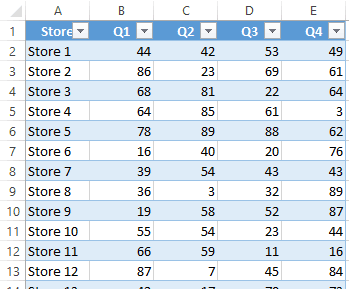
Now I have four workbooks in a folder that I want to combine.
Below is a snapshot of the table I have in one of the workbooks.
Here are the steps to combine the data from these workbooks into a single workbook (as a single table).
- Go to the Data tab.

- In the Get & Transform group, click on the New Query drop down.

- Hover your cursor on ‘From File’ and click on ‘From Folder’.

- In the Folder dialog box, enter the file path of the folder that has the files, or click on Browse and locate the folder.

- Click OK.
- In the dialog box that opens, click on the combine button.

- Click on ‘Combine & Load’.

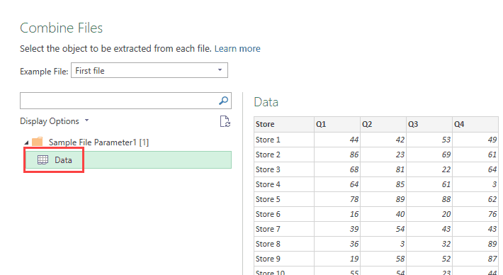
- In the ‘Combine Files’ dialog box that opens, select the Table in the left pane. Note that Power Query shows you the Table from the first file. This file would act as the template (or the key) to combine other files. Power Query would now look for ‘Table 1’ in other workbooks and combine it with this one.

- Click OK.
This will load the final result (combined data) into your active worksheet.
Note that along with the data, Power Query automatically adds the workbook name as the first column of the combined data. This helps in keeping track of what data came from which workbook.
In case you want to first Edit the data before loading it into Excel, in Step 6, select ‘Combine and Edit’. This will open the final result in the Power Query editor where you can edit the data.
A few things to know:
- If you select an Excel Table as the template (in Step 7), Power Query will use the column names in this Table to combine the data from other Tables. If other Tables have additional columns, those will be ignored. In case those other Tables don’t have a column, which is there in your Template Table, Power Query would just put ‘null’ for it.
- The columns don’t need to be in the same order as Power Query uses column headers to map columns.
- Since you have selected Table1 as the key, Power Query will look for Table1 in all the workbooks, and combine all these. In case it doesn’t find an Excel Table with the same name (Table1 in this example), Power Query will give you an error.
Adding New Files to the Folder
Now let’s take a minute and understand what we did with the above steps (which only took us a few seconds).
We combined the data from four different workbooks in one single table in a few seconds without even opening any of the workbooks.
But that’s not all.
The real POWER of Power Query is that now when you add more files to the folder, you don’t need to repeat any of these steps.
All you need to do move the new workbook in the folder, refresh the query, and it will automatically combine the data from all the workbooks in that folder.
For example, in the above example, if I add a new workbook – ‘Mid-West.xlsx’ to the folder, and refresh the query, it will instantly give me the new combined dataset.
Here is how you refresh a query:
- Right-click on the Excel Table that you loaded in the worksheet and click Refresh.

- Right-click on the Query in the ‘Workbook Query’ pane and click Refresh

- Go to the Data tab and click on Refresh.

Each workbook has the data with the same worksheet name
In case you don’t have the data in an Excel Table, but all the sheet names (from which you want to combine the data) are the same, then you can use the method shown in this section.
There are a few things you need to be cautious about when it’s just tabular data and not an Excel Table.
- The worksheet names should be the same. This will help Power Query to go through your workbooks and combine the data from the worksheets that have the same name in each workbook.
- Power Query is case sensitive. This means a worksheet named ‘data’ and ‘Data’ are considered different. Similarly, a column with the header ‘Store’ and one with ‘store’ are considered different.
- While it’s important to have the same column headers, it’s not important to have the same order. If column 2 in the ‘East.xlsx’ is column 4 in ‘West.xlsx’, Power Query will match it correctly by mapping the headers.
Now let’s see how to quickly combine data from different workbooks where the worksheet name is the same.
In this example, I have a folder with four files.
In each workbook, I have a worksheet with the name ‘Data’ that contains the data in the following format (note that this is not an Excel Table).

Here are the steps to combine data from multiple workbooks into one single worksheet:
- Go to the Data tab.
- In the Get & Transform group, click on the New Query drop down.
- Hover your cursor on ‘From File’ and click on ‘From Folder’.
- In the Folder dialog box, enter the file path of the folder that has the files, or click on Browse and locate the folder.
- Click OK.
- In the dialog box that opens, click on the combine button.
- Click on ‘Combine & Load’.
- In the ‘Combine Files’ dialog box that opens, select ‘Data’ in the left pane. Note that Power Query shows you the worksheet name from the first file. This file would act as the key/template to combine other files. Power Query will go through each workbook, find the sheet named ‘Data, and combine all these.
- Click OK. Now Power Query will go through each workbook, look for the worksheet named ‘Data’ in it, and then combine all these datasets.
This will load the final result (combined data) into your active worksheet.
In case you want to first Edit the data before loading it into Excel, in Step 6, select ‘Combine and Edit’. This will open the final result in the Power Query editor where you can edit the data.
Each Workbook has the data with Different Table names or Sheet Names
Sometimes, you may not get structured and consistent data (such as Tables with same name or worksheet with the same name).
For example, suppose you get the data from someone who created these datasets but named the worksheets as East Data, West Data, North Data, and South Data.
Or, the person may have created Excel tables, but with different names.
In such cases, you can still use Power Query, but you need to do it with a couple of additional steps.
- Go to the Data tab.
- In the Get & Transform group, click on the New Query drop down.
- Hover your cursor on ‘From File’ and click on ‘From Folder’.
- In the Folder dialog box, enter the file path of the folder that has the files, or click on Browse and locate the folder.
- Click OK.
- In the dialog box that opens, click on the Edit button. This will open the Power Query editor where you will see the details of all the files in the folder.

- Hold the Control key and select the ‘Content’ and ‘Name’ columns, right-click and select ‘Remove Other Columns’. This will remove all the other columns except the selected columns.

- In the Query Editor ribbon, click on ‘Add column’ and then click on ‘Custom Column’.

- In the Add Custom Column dialog box, name the new column as ‘Data Import’ and use the following formula =Excel.Workbook([CONTENT]). Note that this formula is case sensitive and you need to enter it exactly the way I have shown here.

- Now you will see a new column that has Table written in it. Now let me explain what happened here. You provided Power Query the names of the workbooks, and Power Query has fetched the objects such as worksheets, tables, and named ranges from each workbook (which resides in the Table cell as of now). You can click on the white space next to the text Table and you would see the information at the bottom. In this case, since we only have one table and one worksheet in each workbook, you can see only two rows.
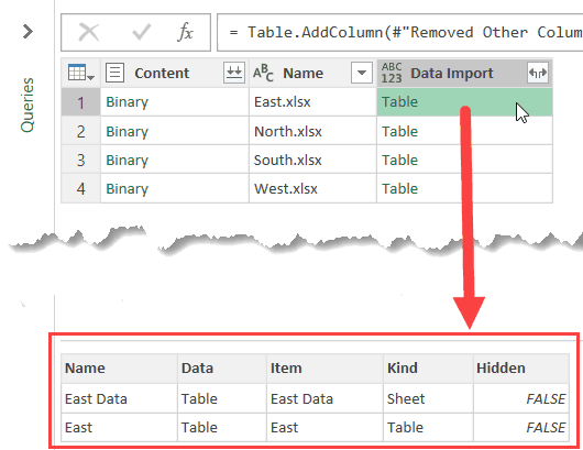
- Click on the double-arrow icon at the top of the ‘Data Import’ column.
- In the column data box that opens, uncheck the ‘Use original column as prefix’, and then click OK.

- Now you will see an expanded table where you see one row for each object in the table. In this case, for each workbook, the sheet object and the table object are listed separately.

- In the Kind column, filter the list to only show the Table.

- Hold the control key and select the Name and Data column. Now, right-click and remove all the other columns.

- In the Data column, click on the double-arrow icon at the top right of the Data Header.
- In the column data box that opens, click OK. This will combine the data in all the tables and show in Power Query.

- Now you can make any transformation you need, and then go to the Home tab and click Close & Load.

Now let me try and quickly explain what we did here. Since there was no consistency in the sheet names or table names, we used the =Excel.Workbook formula to fetch all the objects of the workbooks in the Power Query. These objects can include sheets, tables, and named ranges. Once we had all the objects from all the files, we filtered these to only consider Excel Tables. Then we expanded the data in the tables and combined all these.
In this example, we filtered the data to only use Excel Tables (in Step 13). In case you want to combine sheets and not tables, you can filter sheets.
Note – this technique will give you the combined data even when there is a mismatch in column names. For example, if in East.xlsx, you have a column that has been misspelled, you will end up with 5 columns. Power Query will fill data in columns if it finds it, and if it can not find a column, it will report the value as ‘null’.
Similarly, if you have some additional columns in any of the tables worksheets, these will be included in the final result.
Now if you get more workbooks from which you need to combine data, simply copy-paste it into the folder and refresh the Power Query
You may also like the Following Excel Tutorials:
- Get a List of File Names from Folders & Sub-folders (using Power Query).
- Merge Tables in Excel Using Power Query.
- How to Combine Multiple Excel Files into One Excel Workbook.
- Combine Data From Multiple Worksheets into a Single Worksheet in Excel.
- How to Quickly Combine Cells in Excel.
- How to Select Every Third Row in Excel (or select every Nth Row).
- Split Each Excel Sheet Into Separate Files
- How to Import XML File into Excel | Convert XML to Excel
- Combine CSV Files When Column Headers Don’t Match
- CSV vs XLSX – Key Differences


Dear Sir,
Thank you for sharing the tutorial. It worked properly for me except at one point.
I have a column in the workbooks having data such as 0.5, 1, 2.5
However, after consolidation with above steps, it makes 0.5 as 0, 2.5 as 2.
Thus, it will be very helpful if you can share a solution to the problem.
Sir i have one excel workbook in which i have make 5 sheet region east ,west, north, south and centre and in this data have added .
I want to combine 5 excel sheet data of 1 excel workbook by power query please tell me sir
Dear Sumit,
Firstly, I would like to thank you so much for the excel tips and tutorials.
I’m looking for help in the following scenario.
I have around 50 workbooks. Ex: Company 1, Company 2, 3…and so on…. and a new workbook will be added every week.
And each workbook has a “Table” called “ProductData”.
I have another workbook called “Master Data”.
If I type “Company 1” or “Company 1.xlsx” in the cell ‘A1’ of “Master Data”, the table “ProductData” from “company 1” needs to be imported in cell range starting from ‘A2’.
It has to source the “ProductData” from the file name mentioned in ‘A1’.
It has to be Dynamic.
It has to work without opening the source file.
It also has to source from the new workbooks that may be added to the same folder later.
In simple terms “INDIRECT function without opening the source file”.
Please help me in solving this.
Kindly let me know if you require any more information.
I’m really looking forward to hearing from you.
Thank you so much again for the great excel lessons.
Thanks. It worked and saved my time.
When I refresh all data at the combined file and the source file already open will appear to me a message error that required to close all source files, can I solve this issue without close the files
Hi all,
Please help me i have four different folder like America, Asia, Europe, Pune, Each folder having different files but Same Name and all set of files for two times for Region time refreshed
Example – File Name – Integration log report Co.989 04 PM & Integration log report Co.989 08 AM, same order America, Europe and Pune Region for all Folders.
How to combine all folders files in single file. if possible to take recent files will be okey,
Appreciate your help
That worked perfectly.
I had many files, all with different names, but common sheet names, and I only wanted one sheet out of each file, and this method allowed me to condense them all down to single common sheet.
Brilliant, you are a star!!
Many thanks,
Sam
Thank you so much. Unfortunately I had already manually copied data from 21 files, but looked this up later and tried it and I could have saved even more time. Great tutorial
Great sir, it’s done. Thanks a lot. One problem is that after combining, the query sheet is not editable completely?
What are the limitations to the number of files that can be in a folder? Can there be 1000s of files uploaded?
HI. i follow the step but there is no “combine” option
Thanks A Lot
Hi Sir, Seeking your help.. while consolidated received only one file details…
Will this work if I have shortcuts in one folder or will the actual files need to be in one folder?
nikad ne dofa
As ever, a very useful tutorial! YOu have saved me loads of time (again)
Thank you Sumit
nikad ne dofa