Lookup the Second, the Third, or the Nth Value in Excel

Watch Video – Lookup the Second, the Third or the Nth Matching Value

When it comes to looking up data in Excel, there are two amazing functions that I often use – VLOOKUP and INDEX (mostly in conjunction with the MATCH function).

However, these formulas are designed to find only the first instance of the lookup value.

But what if you want to look-up the second, third, fourth or the Nth value.

Well, it’s doable with a little bit of extra work.

In this tutorial, I will show you various ways (with examples) on how to look up the second or the Nth value in Excel.

Lookup the Second, Third, or Nth Value in Excel

In this tutorial, I will cover two ways to look-up the second or the Nth value in Excel:

• Using a helper column.
• Using array formulas.

Let’s get started and dive right in.

Using Helper Column

Suppose you are a training coordinator in an organization and have a dataset as shown below. You want to list all the training in front of an employee’s name.

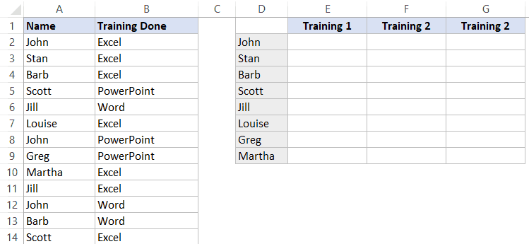
In the above dataset, the employees have been given training on different Microsoft Office tools (Excel, PowerPoint, and Word).

Now, you can use the VLOOKUP function or the INDEX/MATCH combo to find the training an employee has completed. However, it will only return the first matching instance.

For example, in the case of John, he has taken all the three training, but when I look up his name with VLOOKUP or INDEX/MATCH, it will always return ‘Excel’, which is the first training for his name in the list.

To get this done, we can use a helper column and create unique lookup values in it.

Here are the steps:

• Insert a column before the column that lists the training.
• In cell B2, enter the following formula:

  =A2&COUNTIF($A$2:$A2,A2)

• In cell F2, enter the following formula and copy-paste for all the other cells:

  =IFNA(VLOOKUP($E2&COLUMNS($F$1:F1),$B$2:$C$14,2,0),"")

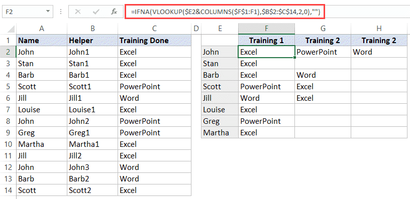
The above formula would return the training for each employee in the order it appears on the list. In case there are no training listed for an employee, it returns a blank.

How does this formula work?

The COUNTIF formula in the helper column makes each employee’s name unique by adding a number to it. For example, the first instance of John becomes John1, the second instance becomes John2 and so on.

The VLOOKUP formula now uses these unique employee names to find the matching training.

Note that $E2&COLUMNS($F$1:F1) is the lookup value in the formula. This would add a number to the employee name based on the column number. For example, when this formula is used in cell F2, the lookup value becomes “John1”. In cell G2, it becomes “John2” and so on.

Using  Array Formula

If you don’t want to alter the original dataset by adding helper columns, you can also use an array formula to look up the second, third, or the nth value.

Suppose you have the same dataset as shown below:

Here is the formula that will return the correct lookup value:

=IFERROR(INDEX($B$2:$B$14,SMALL(IF($A$2:$A$14=$D2,ROW($A$2:$A$14)-1,""),COLUMNS($E$1:E1))),"")

Copy this formula and paste it in cell E2.

Note that this is an array formula and you need to use Control + Shift + Enter (hold the Control and Shift keys and press the Enter key), instead of hitting just the Enter key.

Click here to download the example file.

How does this formula work?

Let’s break this formula into parts and see how it works.

$A$2:$A$14=$D2

The above part of the formula compares each cell in A2:A14 with the value in D2. In this dataset, it checks whether a cell contains the name “John” or not.

It returns an array of TRUE of FALSE. If the cell has the name ‘John’ it would be True, else it would be False.

Below is the array you would get in this example:

{TRUE;FALSE;FALSE;FALSE;FALSE;FALSE;TRUE;FALSE;FALSE;FALSE;TRUE;FALSE;FALSE}

Note that it has TRUE in 1st, 7th and 111th position, as there is where the name John appears in the dataset.

IF($A$2:$A$14=$D2,ROW($A$2:$A$14)-1,””)

The above IF formula uses the array of TRUE and FALSE, and replaces TRUE with the position of its occurrence in the list (given by ROW($A$2:$A$14)-1) and FALSE with “” (blanks). The following is the resulting array you get with this IF formula:

{1;””;””;””;””;””;7;””;””;””;11;””;””}

Note than 1, 7, and 11 are the position of occurence of John in the list.

SMALL(IF($A$2:$A$14=$D2,ROW($A$2:$A$14)-1,””),COLUMNS($E$1:E1))

The SMALL function now picks the first smallest, second smallest, third smallest number from this array. Note that it uses the COLUMNS function to generate the column number. In cell E2, the COLUMNS function returns 1 and the SMALL function returns 1. In cell F2, COLUMNS function returns 2 and the SMALL function returns 7.

INDEX($B$2:$B$14,SMALL(IF($A$2:$A$14=$D2,ROW($A$2:$A$14)-1,””),COLUMNS($E$1:E1)))

INDEX function now returns the value from the list in Column B based on the position returned by the SMALL function. Hence, in cell E2, it returns ‘Excel’, which is the first item in B2:B14. In cell F2, it returns PowerPoint, which is the 7th item in the list.

Since there are cases where there are only one or two training for some employees, INDEX function would return an error. The IFERROR function is used to return a blank in place of the error.

Note that in this examples, I have used range references. However, in practical examples, it’s beneficial to convert he data into an Excel Table. By converting into an Excel Table, you can use structured references, which makes it easier to create formulas. Also, an Excel Table can automatically account for any new training items that are added to the list (so you don’t have to adjust the formulas every time).

What do you do when you have to look-up the second, third, or the Nth value? I am sure there are more ways to do this. If you use something easier than the one listed here, do share with us all in the comments section.

Click here to download the example file.

You May Also Like the Following Excel Tutorials:

• VLOOKUP vs INDEX/MATCH.
• INDEX MATCH Combo in Excel (examples)
• How to make VLOOKUP Case Sensitive.
• How to Use VLOOKUP with Multiple Criteria.
• Use IFERROR with VLOOKUP to Get Rid of #N/A Errors
• Find the Second Highest Value in Excel