Excel Filter Function – Explained with Examples + Video

Watch Video – Excel FILTER Function Examples

Office 365 brings with some awesome functions – such as XLOOKUP, SORT, and FILTER.

When it comes to filtering data in Excel, in the pre-Office 365 world, we were mostly dependent on Excel in-built filter or at max the Advanced filter or complex SUMPRODUCT formulas. In case you had to filter a part of a dataset, it was usually a complex workaround (something I have covered here).

But with the new FILTER function, it’s now really easy to quickly filter part of the dataset based on a condition.

And in this tutorial, I will show you how awesome is the new FILTER function and some useful things you can do with this.

But before I get into the examples, let’s quickly learn about the syntax of the FILTER function.

Excel Filter Function – Syntax

Below is the syntax of the FILTER function:

=FILTER(array,include,[if_empty])

• array – this is the range of cells where you have the data and you want to filter some data from it
• include – this is the condition that tells the function what records to filter
• [if_empty] – this is an optional argument where you can specify what to return in case no results are found by the FILTER function. By default (when not specified), it returns the #CALC! error

Now let’s have a look at some amazing Filter function examples and stuff it can do which used to be quite complex in its absence.

Click here to download the Example file and follow along

Example 1: Filtering Data Based on One Criteria (Region)

Suppose you have a dataset as shown below and you want to filter all the records for the US only.

Below is the FILTER formula that will do this:

=FILTER($A$2:$C$11,$B$2:$B$11="US")

The above formula uses the dataset as the array and the condition is $B$2:$B$11=”US”

This condition would make the FILTER function check every cell in column B (one that has the region) and only those records that match this criterion would be filtered.

Also, in this example, I have the original data and the filtered data on the same sheet, but you can also have these in separate sheets or even workbooks.

Filter Function returns a result that is a dynamic array (which means that instead of returning one value, it returns an array that spills to other cells).

For this to work, you need to have an area where the result would come to be empty. In any of the cells in this area (E2:G5 in this example) already has something in it, the function will give you the #SPILL error.

Also, since this is a dynamic array, you can not change a part of the result. You can either delete the entire range that has the result or cell E2 (where the formula was entered). Both of these would delete the entire resulting array. But you can not change any individual cell (or delete it).

In the above formula, I have hard-coded the region value, but you can also have it in a cell and then reference that cell that has the region value.

For example, in the below example, I have the region value in cell I2 and this is then referenced in the formula:

=FILTER($A$2:$C$11,$B$2:$B$11=I1)

This makes the formula even more useful, and now you can simply change the region value in cell I2, and the filter would automatically change.

You can also have a drop-down in cell I2 where you can simply make the selection and it would instantly update the filtered data.

Also read: Excel LAMBDA Function

Example 2: Filtering Data Based on One Criteria (More Than or Less Than)

You can also use comparative operators within the filter function and extract all the records that are more or less than a specific value.

For example, suppose you have the dataset as shown below and you want to filter all the records where the sales value is more than 10000.

The below formula can do this:

=FILTER($A$2:$C$11,($C$2:$C$11>10000))

The array argument refers to the entire dataset and the condition, in this case, is ($C$2:$C$11>10000).

The formula checks each record for the value in Column C. If the value is more than 10000, it is filtered, else it’s ignored.

In case you want to get all the records less than 10000, you can use the below formula:

=FILTER($A$2:$C$11,($C$2:$C$11<10000))

You can also get more creative with the FILTER formula. For example, if you want to filter the top three record based on the sales value, you can use the below formula:

=FILTER($A$2:$C$11,($C$2:$C$11>=LARGE(C2:C11,3)))

The above formula uses the LARGE function to get the third largest value in the dataset. This value is then used in the FILTER function criteria to get all the records where the sales value is more than or equal to the third-largest value.

Click here to download the Example file and follow along

Example 3: Filtering Data with Multiple Criteria (AND)

Suppose you have the below dataset and you want to filter all the records for the US where sale value is more than 10000.

This is an AND condition where you need to check for two things – the region needs to the US and the sales need to be more than 10000. If only one condition is met, the results should not be filtered.

Below is the FILTER formula that will filter records with the US as the region and sales of more than 10000:

=FILTER($A$2:$C$11,($B$2:$B$11="US")*($C$2:$C$11>10000))

Note that the criterion (called the include argument) is ($B$2:$B$11=”US”)*($C$2:$C$11>10000)

Since I am using two conditions and I need both to be true, I have used the multiplication operator to combine these two criteria. This returns an array of 0’s and 1’s, where a 1 is returned only when both the conditions are met.

In case there are no records that meet the criteria, the function would return the #CALC! error.

And in case you want to return something meaning (instead of the error), you can use a formula as shown below:

=FILTER($A$2:$C$11,($B$2:$B$11="USA")*($C$2:$C$11>10000),"Nothing Found")

Here, I have used “Not Found” as the third argument, which is used when no records are found that match the criteria.

Example 4: Filtering Data with Multiple Criteria (OR)

You can also modify the ‘include’ argument in the FILTER function to check for an OR criteria (where any one of the given conditions can be true).

For example, suppose you have the dataset as shown below and you want to filter the records where the country is either the US or Canada.

Below is the formula that will do this:

=FILTER($A$2:$C$11,($B$2:$B$11="US")+($B$2:$B$11="Canada"))

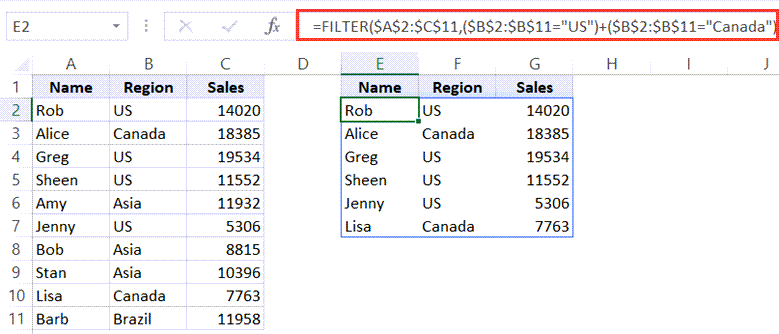
Note that in the above formula, I have simply added the two conditions by using the addition operator. Since each of these conditions returns an array of TRUEs and FALSEs, I can add to get a combined array where it’s TRUE if any one of the conditions is met.

Another example could be when you want to filter all the records where either the country is the US or the sale value is more than 10000.

The below formula will do this:

=FILTER($A$2:$C$11,($B$2:$B$11="US")+(C2:C11>10000))

Note: When using AND criteria in a FILTER function, use the multiplication operator (*) and when using the OR criteria, use the addition operator (+).

Example 5: Filtering Data To Get Above/Below Average Records

You can use formulas within the FILTER function to filter and extract records where the value is above or below the average.

For example, suppose you have the dataset as shown below and you want to filter all the records where the sale value is above average.

You can do that using the following formula:

=FILTER($A$2:$C$11,C2:C11>AVERAGE(C2:C11))

Similarly, for below average, you can use the below formula:

=FILTER($A$2:$C$11,C2:C11<AVERAGE(C2:C11))

Click here to download the Example file and follow along

Example 6: Filtering Only the EVEN Number Records (Or ODD Number Records)

In case you need to quickly filter and extract all the records from even number rows or odd number rows, you can do that with the FILTER function.

To do this, you need to check the row number within the FILTER function, and only filter row numbers that meet the row number criteria.

Suppose you have the dataset as shown below and I only want to extract even-numbered records from this dataset.

Below is the formula that will do this:

=FILTER($A$2:$C$11,MOD(ROW(A2:A11)-1,2)=0)

The above formula uses the MOD function to check the row number of each record (which is given by the ROW function).

The formula MOD(ROW(A2:A11)-1,2)=0 returns TRUE when the row number is even and FALSE when it’s odd. Note that I have subtracted 1 from the ROW(A2:A11) part as the first record is in the second row, and this adjusts the row number to consider the second row as the first record.

Similarly, you can filter all the odd-numbered records using the below formula:

=FILTER($A$2:$C$11,MOD(ROW(A2:A11)-1,2)=1)

Example 7: Sort the Filtered the Data With Formula

Using FILTER function with other functions allows us to get a lot more done.

For example, if you filter a dataset using the FILTER function, you can use the SORT function with it to get the result that is already sorted.

Suppose you have a dataset as shown below and you want to filter all the records where the sales value is more than 10000. You can use the SORT function with the function to make sure the resulting data is sorted based on the sales value.

The below formula will do this:

=SORT(FILTER($A$2:$C$11,($C$2:$C$11>10000)),3,-1)

The above function uses the FILTER function to get the data where the sale value in column C is more than 10000. This array returned by the FILTER function is then used within the SORT function to sort this data based on the sales value.

The second argument in the SORT function is 3, which is to sort based on the third column. And the fourth argument is -1 which is to sort this data in descending order.

Click here to download the Example file

So these are 7 examples to use the FILTER function in Excel.

Hope you found this tutorial useful!

You may also like the following Excel tutorials:

1. How to Filter Cells with Bold Font Formatting in Excel
2. Filter By Color in Excel
3. Dynamic Excel Filter Search Box
4. How to Filter Data in a Pivot Table in Excel