How to Filter Cells with Bold Font Formatting in Excel (An Easy Guide)

I get this query all the time. People have huge data sets and someone in their team has highlighted some records by formatting it in bold font.

Now, you are the one who gets this data, and you have to filter all these records that have a bold formatting.

For example, suppose you have the data set as shown below, and you want to filter all the cells that have been formatted in bold font.

Let’s face it.

There is no straightforward way of doing it.

You cannot simply use an Excel filter to get all the bold cells. But that doesn’t mean you have to waste hours and do it manually.

In this tutorial, I will show you three ways to filter cells with bold font formatting in Excel:

Method 1 – Filter Bold Cells Using Find and Replace

Find and Replace can be used to find specific text in the worksheet, as well as a specific format (such as cell color, font color, bold font, font color).

The idea is to find the bold font formatting in the worksheet and convert it into something that can be easily filtered (Hint: Cell color can be used as a filter).

Here are the steps filter cells with bold text format:

1. Select the entire data set.
2. Go to the Home tab.
3. In the Editing group, click on the Find and Select drop down.
4. Click on Replace. (Keyboard shortcut: Control + H)
5. In the Find and Replace dialog box, click on the Options button.
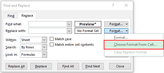
6. In the Find what section, go to the Format drop-down and select ‘Choose Format From Cell’.
7. Select any cell which has the text in bold font format.
8. In the ‘Replace with:’ section, go to Format drop-down and click on ‘Choose Format From Cell’ option.
9. In the Replace Format dialog box, select the Fill Tab and select any color and click OK (make sure it’s a color that is not there already in your worksheet cells).
10. Click on Replace All. This will color all the cells that have the text with bold font formatting. 

In the above steps, we have converted the bold text format into a format that is recognized as a filter criterion by Excel.

Now to filter these cells, here are the steps:

1. Select the entire data set.
2. Go to the Data tab.
3. Click on the Filter icon (Key Board Shortcut: Control + Shift + L)
4. For the column that you want to filter, click on the filter icon (the downward pointing arrow in the cell).
5. In the drop-down, go to the ‘Filter by Color’ option and select the color you applied to cells with text in bold font format.

This will automatically filter all those cells that have bold font formatting in it.

Try it yourself.. Download the file

Method 2 – Using Get.Cell Formula

It time for a hidden gem in Excel. It’s an Excel 4 macro function – GET.CELL().

This is an old function which does not work in the worksheet as regular functions, but it still works in named ranges.

GET.CELL function gives you the information about the cell.

For example, it can tell you:

• If the cell has bold formatting or not
• If the cell has a formula or not
• If the cell is locked or not, and so on.

Here is the syntax of the GET.CELL formula

=GET.CELL(type_num, reference)

• Type_num is the argument to specify the information that you want to get for the referenced cell (for example, if you enter 20 as the type_num, it would return TRUE if the cell has a bold font format, and FALSE if not).
• Reference is the cell reference that you want to analyze.

Now let me show you how to filter cells with text in a bold font format using this formula:

1. Go to Formulas tab.
2. Click on the Define Name option.
3. In the New Name dialog box, use the following details:
   • Name: FilterBoldCell
   • Scope: Workbook
   • Refers to: =GET.CELL(20,$A2)
4. Click OK.
5. Go to cell B2 (or any cell in the same row as that of the first cell of the dataset) and type =FilterBoldCell
6. Copy this formula for all the cell in the column. It will return a TRUE if the cell has bold formatting and FALSE if it does not.
7. Now select the entire data set, go to the Data tab and click on the Filter icon.
8. In the column where you have TRUE/FALSE, select the filter drop-down and select TRUE.

That’s it!

All the cells with text in bold font format have now been filtered.

Note: Since this is a macro function, you need to save this file with a .xlsm or .xls extension.

I could not find any help article on GET.CELL() by Microsoft. Here is something I found on Mr. Excel Message Board.

Try it yourself.. Download the file

Method 3 – Filter Bold Cells using VBA

Here is another way of filtering cells with text in bold font format by using VBA.

Here are the steps:

1. Right-click on the worksheet tab and select View Code (or use the keyboard shortcut ALT + F11). This opens the VB Editor backend.
2. In the VB Editor window, there would be the Project Explorer pane. If it is not there, go to View and select Project Explorer.
3. In the Project Explorer pane, right click on the workbook (VBAProject) on which you are working, go to Insert and click on Module. This inserts a module where we will put the VBA code.
4. Double click on the module icon (to make sure your code into the module), and paste the following code in the pane on the right:

   Function BoldFont(CellRef As Range)
   BoldFont = CellRef.Font.Bold
   End Function

5. Go to the worksheet and use the below formula: =BoldFont(B2)
6. This formula returns TRUE wherever there is bold formatting applied to the cell and FALSE otherwise. Now you can simply filter all the TRUE values (as shown in Method 2)

Again! This workbook now has a macro, so save it with .xlsm or .xls extension

Try it yourself.. Download the file

I hope this will give you enough time for that much-needed coffee break 🙂

Do you know any other way to do this? I would love to learn from you. Leave your thoughts in the comment section and be awesome.

You May Also Like the Following Excel Tutorials:

• An Introduction to Excel Data Filter Options.
• Filter By Color in Excel
• Create Dynamic Excel Filter – Extract Data as you type.
• Creating a Drop Down Filter to Extract Data Based on Selection.
• Filter the Smart Way – Use Advanced Filter in Excel
• Count Cells Based on a Background Color.
• Highlight Blank Cells in Excel.
• How to Create a Heat Map in Excel.
• Excel VBA Autofilter.