
In this tutorial, I will show you how to create a drop-down filter in Excel so that you can extract data based on the selection from the drop-down.
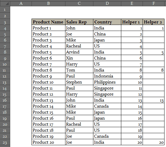
As shown in the pic below, I have a created a drop-down list with country names. As soon as I select any country from the drop-down, the data for that country gets extracted to the right.
Note that as soon as I select India from the drop-down filter, all the records for India are extracted.

Extract Data from Drop Down List Selection in Excel
Here are the steps to create a drop-down filter that will extract data for the selected item:
- Create a Unique list of items.
- Add a drop-down filter to display these unique items.
- Use helper columns to extract the records for the selected item.
Let’s deep dive and see what needs to be done in each of these steps.
Create a Unique List of Items
While there could be repetitions of an item in your dataset, we need unique item names so that we can create a drop down filter using it.
In the above example, the first step is to get the unique list of all the countries.
Here are the steps to get a unique list:
- Select all the Countries and paste it at some other part of the worksheet.
- Go to Data –> Remove Duplicates.
- In the Remove Duplicates dialogue box, select the column where you have the list of countries. This will give you a unique list as shown below.

Now we will use this unique list to create the drop-down list.
See Also: The Ultimate Guide to Find and Remove Duplicates in Excel.
Creating the Drop Down Filter
Here are the steps to create a drop down list in a cell:
- Go to Data –> Data Validation.
- In Data Validation dialogue box, select the Settings tab.
- In Settings tab, select “List” in the drop down, and in ‘Source’ field, select the unique list of countries that we generated.
- Click OK.

The goal now is to select any country from the drop-down list, and that should give us the list of records for the country.
To do this, we would need to use helper columns and formulas.
Create Helper Columns to Extract the Records for the Selected Item
As soon as you make the selection from the drop down, you need Excel to automatically identify the records that belong to that selected item.
This can be done using three helper columns.
Here are the steps to create helper columns:
- Helper Column #1 – Enter the serial number for all the records (20 in this case, you can use ROWS() function to do this).
- Helper Column #2 – Use this simple IF Function function: =IF(D4=$H$2,E4,””)
- This formula checks whether the country in the first row matches the one in the drop down menu. So if I select India, It checks whether the first row has India as the country or not. If it’s True, it returns that row number, else it returns blank (“”). Now when we select any country, only those row numbers are displayed (in the second helper column) which has the selected country in it. (For example, if India is selected, then it will look like the pic below).
 Now we need to extract the data for these rows only, which displays the number (as it is the row that contains that country). However, we want those records without the blanks one after the other. This can be done using a third helper column
- Third Helper Column – Use the following combination of IFERROR and SMALL functions: =IFERROR(SMALL($F$4:$F$23,E4),””)
This would give us something as shown below in the pic:
 Now when we have the number together, we just need to extract the data in that number. This can be done easily using the INDEX function (use this formula in the cells where you need the result extracted):
=IFERROR(INDEX($B$4:$D$23,$G4,COLUMNS($J$3:J3)),””)
This formula has 2 parts:
INDEX – This extracts the data based on the row number
IFERROR – This function returns blank when there is no data
Here is a snapshot of what you finally get:

You can now hide the original data if you want. Also, you can have the original data and extracted data in two different worksheets as well.
Go ahead. use this technique, and impress your boss and colleagues (a little show-off is never a bad thing).
Download the Example File
Did you like the tutorial? Let me know your thoughts in the comments section.
You May Also Find the Following Tutorials Useful:


While put the formula in Helper 3 getting a #NAME? error.
Please help.
Does anyone know how I could do this, but add a second filter in addition to the first? Ie. I want to filter for India and then within what’s filtered for India I want to also filter by Sales Rep name?
This tutorial was extraordinarily helpful in demonstrating this technique and enabling me to accomplish a specific task I was trying to complete. Thank you!
Hi Sumit,
Thank you for your tutorial, I have used your technique last year in an attendance sheet by creating a drop down list with department names and then it lists the staff name and ID. I have created the helper table on each tab of the sheet representing the year and using the drop down list of each sheet.
My problem is when adding newly hire employee or removing retired employee i have to make it manually on each sheet.
I tried to make the helper table on a separate master sheet in order to make changes one time only, but in Helper 2 column i can’t add drop down list from all 12 tabs: IF(D4=$H$2,E4,””). I mean instead of $H$2, add ‘June20′! $C3:’July 21’!$C3
Is there a away to show you the sheet and help me to have more than one drop down list in the formula of Helper
Thank you 2.
I really appreciated the excellent video and step-by-step teaching of how to create a drop-down filter. My question: Is there a way to add a “Show All” to the drop-down filter so that all filtered data in the table becomes visible? Or, have the data table already populated when the worksheet is first open then use the drop-down filter to filter the data in the same table? Thanks.
Very helpful.This is I wanted for a long time. Based on this video I created a table.In the unique list there are names like Sandiya and Balasandiya. When I extract the details for Sandiya, the details for Balasandiya are also extracted but not in vice versa.How to correct it? Please help me.
Hey mate. Love your Excel tips. Cheers
Hi Sumit okay lets start at A. I have two sheets, data sheet and main sheet. on main sheet I have drop down on cell D6 with values that match the values in row 8 on data sheet. If any value is true I want that complete column to be returned on main page. There could be up to 4 values that could match any of the values matched in row 8 on data sheet. My first attempt was with this: =IFERROR(INDEX(Inverter!$C$2:$T$15;;Inverter!C$19;ROWS(Inverter!$C$21:C$21));””), this works okay but only return the value of row 2 even with drag across all 4 columns match but only with top row. As soon as I drag the formula down the same value as in the top cell of each column return.
Hi Sumit,
I’m struggling to work out which formulas I need to be using.
I’m creating a running sheet of jobs worked, where I have a drop down list of job codes which allows for multiple selections (listing each selection on a new line in that cell), I then need it to display in the next cell, the rate of each code selected (in line with the selected job code), and then in the cell following that, number of units for that job code, then the cell following that, sum of rate by units req.
please help.
I can send you a file of where I’m currently at, please let me know where to send it.
regards
Steve
Hi sumit, Is there any way of showing all items in a product which is in dropdown list?
Greetings Sumit, I’m completely stumped, I’m trying to do this in the opposite direction. I have a Row which will be the main position of the primary selector. After selecting which item in the drop box i need; rather than having the information populate in different columns; I need the extractor to populate the data beneath that primary select in the same row and create additional rows if possible. I have a visual representation of what I need; is this even possible? Please respond.
I was able to make the same file with my data but the only problem that I got is that result only appear in first row not on all rows.
Dear sir, when i make like this including date format and number, My answer is wrong. How to do this. Can i send you my file. Thanks
I follow all the steps but when i my country in the drop down list menu – it did not populate with country selected
Brilliant tip. Did just what I wanted.
This is great! How can I achieve this same result for a comma delimited column?
Thank you very much, this was the best lesson I have seen! However, I have a little different challenge and I need to add multiple dropdown selections and produce a consolidated list of only correct matches. Can you please help me?
I need this too
How do I repeat this on the next drop down with the same information needed? I’m using it to pull equipment used on a test.
I’ve used your method and got what i want, but I need some more help, as I’ve a ledger of some consumers which contains some data like consumer name, consumer number (unique number), city, and area or street they live. I want to extract filtered data using more than one dependent drop down list, 1st one is “city” and another one is “area or street they live in”. what to do?
if i use the above example, i only get one type of data which is dependent on “area or street they live in, but i wanted to filter it out with both city and street…
plz help me..
Hi Sumit
Great tutorial. It works a treat.
I have an issue; if a record (row)on a separate data worksheet is deleted or inserted, the helper1 and 2 columns receive a #REF error as the reference is broken. I tried a number of solutions but couldn’t get it to work. I have ended up protecting rows and columns in the sheet. Any ideas?
Thanks again.
Hi Everyone,
I need a favor of yours. I have just implemented the same into Google spreadsheet and it’s creating an issue. I and created the same in Excel and it’s working fine.
In google sheet, the logic =IFERROR(INDEX(Data!$A$4:$C$52,Data!F4,1),””) is not working especially when there is no reference instead of printing blank it’s breaking.
Please let me know if you have any solution here.
Thanks in advance.
Hello, I have an excel sheet with multiple columns containing different information. In the drop down list for each column, multiple values can be selected. How do I pull data from a drop down list with multiple values?
Hi – I have found your tutorial really interesting and easy to follow / use.
I’m now wondering if there is a way to link 2 or more drop down lists for one data table to dynamically update based on options selected within multiple down lists. I’m guessing there must be a way to amend the following formula “=INDEX(‘Table1′!$F$7:$L$5654,’Table1’!$N7,COLUMNS($G$8:G8))” to expand on the dropdown lists used to update the data tables.
Are you able to advise how I should go about achieving this or point me in the right direction of where I can find tutorials around this please?
Any help / advise would be greatly appreciated.
Many thanks, Mike.
V. Helpful and just what I was looking for. One question: if, using your example, the sales reps covered multiple countries how could you filter in that case? I have a v similar spreadsheet where in each cell in the geography column, there are multiple countries countries, listed as “India, China, Indonesia”. I need to be able to filter by one country. Would there be a way of filtering by country without delimiting the countries into separate cells? Thanks!!
Hii..Very helpful excel functionalities..The steps helped me to develop a report completely.
Thanks.
Hi! Thanks for sharing this, really helpful. Also, if I have to create three unique drop-down lists and pull data from source sheet automatically based on the drop-down selection. Say have data by industry, by geography and by month, now need to pull information by a combination of this 3 filters from unique drop-down lists. Can you help?
Almost exactly what I’ve been looking for. Thank you.
How do I add multiple drown down menus? For example,
If i wanted a drop down menu for Geography and product name?
Hi Guys, I’m stumped with this one. I’m using the following formula to get the helper 3 coloumn. It works fine for a small array of 1000 rows, but when I increase it to 10,000 for example…. it returns BLANK? – Any Ideas?
=IFERROR(SMALL($Q$2:$Q$1048,ROWS($Q$2:Q2)),””)
Hi Guys, I’m stumped with this one. I’m using the following formula in column E to return the row numbers of the name I’ve selected in column A, to get the helper 3 bit. It works fine for a small array of 1000 rows, but when I increase it to 10,000 for example…. it returns BLANK? – Any Ideas?
=IFERROR(SMALL($Q$2:$Q$1048,ROWS($Q$2:Q2)),””)
HI, nice tutorial, but i was made for 3 column, what if i have around 12 columns, how many helper i will create?
Hello, How would the formula change on the helper columns if I’m trying to extract several columns of data. For example if I need 6 columns extracted would I need 6 helpers columns and what formulas would change?
Thank you!
Helper column is not how many columns of data you are extracting rather they are there to help finding row numbers from the data needs to be extracted.
Now from how many columns you have you can use array formula if more by selecting the columns and enter formula, then enter ALT+CTRL+ENTER
you will see { } brackets in formula bar that will extract all the columns data in one go
Hello! is it possible for the drop down list to be multiple selection? how do i extract multiple data if i have more than one selection from the list?
Hi, thank you for this!
I just have one more question, what if i want to add one more column after sales rep column, what is the formula for that?
thanks
Do you know how to do this through Google Sheets?
Does this pull from multiple sheets? I’d like to get a drop down to reference several sheets of values on the last page so people can see all the data relative to their names and save searching time, but there are multiple sheets worth of data to track, and compiling them into one document makes my work significantly harder.
Wow… this works perfectly.
Thanks a bunch.
I have a multiple drop down it has the match all the drop down and fetch the data Please help. I am able to use only one drop down to fetch the data as explained above
Can anyone please help me with the below query?
My requirement is… when i select a value on column A, then column B should list only the values related to Column A
ColumnA ColumnB
123 1
123 2
234 1
234 2
345 1
456 1
567 1
678 1
Expected Result
ColumnA (drop down) ColumnB (drop down)
123 1
2
Hi Sumit,
Hope you can help me with this..
My requirement is… when i select a value on column A, then column B should list only the values related to Column A
ColumnA ColumnB
123 1
123 2
234 1
234 2
345 1
456 1
567 1
678 1
Expected Result
ColumnA (drop down) ColumnB (drop down)
123 1
2
Thank you for this solution.
IS this able to be done in Google Sheets?
Thank you
Thanks so much. This tutorial helped me improve our processes and productivity. Looking forward to doing so much more with Excel now. (They should pay you!)
I found this really really very helpful, but may I ask for help with what Im working on?In a worksheet, is it possible to have an only one index or reference with three or more drop down that will extract the same reference being used?
Hi! this is so great thanks! Is there a way I can add one more drop down list criteria? So for example in your tutorial. I select India and get data extracted for India, but what if i want India AND only sales rep Joe. SO i would have a drop down list for India and another drop down list to just look at sales rep Joes stuff?
i know youve answered this but i dont know how to adjust my helper column to make sure that it returns true after two criteria are met
Have a look at this: https://www.dropbox.com/s/4kdooaij0ch5lvu/Extarct%20Data%202%20conditions_Custom-Filter.xls?dl=0
Hey Ashley, Have a look at this: https://www.dropbox.com/s/4kdooaij0ch5lvu/Extarct%20Data%202%20conditions_Custom-Filter.xls?dl=0
How can i also incorporate ALL meaning just show me ALL for country and ALL for sales rep?
Hi Sumit, can you do this so it is not AND. I want mutliple drop down boxes and it only picks up to seach if some is selected. ie if i pick country and sales rep it shows only when both but if i just pick country the list still populates
is there a way to have a searchable drop down list? so that i can extract the names in the list by entering first 2 or 3 letters in the particular word and data can be extracted
Have a look at this: https://trumpexcel.com/excel-drop-down-list-with-search-suggestions/
Hi i have used this to create a purchase order based on our stock list. It works brilliantly, except i would like it to only show rows of, In my case, items to order with a quantity of 1 and above how can i do this. Thank you
Can we extract the data from multiple drop-down selection?
Yes you can extract using multiple drop downs as well. You’ll need to modify the condition in helper column such that it returns TRUE only when all the drop down selection match
OK…could you share an example please?
Can I have an excel sheet with all the data from the drop down selections on it without the drop down?
Hello Karl.. Yes you can have it on a different sheet. If you’re looking to get static data, you can also use Advanced filter (http://trumpexcel.com/2013/08/advanced-filter-in-excel-some-cool-tricks/)
Hi, if one product is shared by two countries how can I filter that ?
Hi,
Request you to please share same process in VBA code.
Email.id : sachin.nikam@hungama.com
Hello there!
Thank you so much for your explanation, it is great!
I am using a file which doesn’t bring country list; however, brings some information other spreadsheet. Anyway it is not working, the “helper 3” brings the information, but doesn’t show up on “Product name or Sales Rep” and I do not know what I made wrong.
Can you please help me? I really got stuck on these files, 2 weeks already 🙁
Thank you,
Cris
I forgot the file!
Thank you!
greetings trump excel.com it is great platform to learn best excel warm greetings and thanks to all excel bestie’s here in this list….m here suppose to ask question but i see lawre*** has already ask the same question question thanks to Mr. sumit bansal for great help!!!!!
shaikh imran
This has helped! But I do have a question (apologies if this
has already been answered in the comments).
I am having a problem with cross referencing the data. For example I want to
see all the people from a certain district and then filter the results by how
many male/female in that district. When I try this it doesn’t work, I believe
it has something to do with the ‘helper’ columns. Do you know how to make this
work?
Thanks a lot, this is amazing!
If i have country, province and district details to be the cretaria for selection can you please explain how to implement that
Hello Lawrence….how do i do this with lots of data
Hi if I want to add a row into the data like example I want to insert an additional product between product 14 and product 15, the helpers do not update automatically. What can I do to make the helpers update automatically when a row is added / deleted? So that the extracted data on the right shows the new data?
Once you have inserted a new row, click on the first cell of each column. When you click on the cell you will see a small black square at the bottom right. Click on it and drag it down. Do it for all the columns.
Hi! Great tutorial.
I’m trying to make a excel sheet with product information witch can sort out and display products witch match certain criteria. Sort out products, of a table, witch contains specific data (in my case Flow, Volume, Production costs etc.). My goal is to have a worksheet with my company’s old work (I work with water cleaning systems) and with this worksheet sort out all the water cleaning systems witch match my search, and display those in some way. And then automaticly calculate a price based on those. I want to able to have multiple drop downs to make my search narrower.
I have tried slicers but i can’t get it to work and display multiple matches. Maybe it’s easier with drop down lists?
Hello Erik.. It would be helpful if you could share a sample data file.
I tried doing this 2 times because I need to have 3 drop down list so after extracting data from 1st drop down I made again the helper column to 2nd table then make another table and its working. but my problem is, I want to make my drop down list dependent on what 1st drop down list chose then 2nd drop down list to 3rd drop down list. I tried following the dependent drop down list tutorial but it’s not working. please help me to make this 3 drop down list dependent to each other after extracting data from one another. Or is there any way to do this. thanks
Hello.. Can you share the sample file. It would be easier to guide once I can see the data
Hi, in your spreadsheet I would like to add 2 additional drop down boxes for Sales Rep then Product Name. I want each drop down to be dependent on the first drop down boxes criteria. How can I make this possible?
Great tutorial!! These lessons keep opening new ideas for existing files I work with to make them better. I do need to manipulate the data from this lesson once more. I have a database that lists as columns: First name, Last name Floor, Cubicle, Job Position, Training Date, Equipment issued, issued date. When data is entered I have drop down menus for Job position and Equipment issued. Multiple equipment can be issued to the same person which creates blank cells in the other columns until another name is entered. On the next sheet I have the sort by drop down list as mentioned above. I have successfully implemented it and even get the blank lines to be ignored. However, I need that sorted table, or the first one, to be listed alphabetically by LAST NAME automatically. I cannot sort the first database by last name as the blank lines will not properly adjust with the associated name. Basically I need to sort alphabetically Helper column 3 from above or the main database taking in to account the blank cells.
Hi….Is there is possibility to Add more 3 or 4 columns along with Product Name, Sales Representative and Geography ?. If, Yes, Kindly request you please add 4 columns. Waiting for your new editions.
I guesst this is the formula I’ve tried:
=IFERROR(INDEX(‘DUES MTH 1′:’DUES MTH 12′!$E$4:’DUES MTH 1′:’DUES MTH 12′!$AI$68,’DUES MTH 1′:’DUES MTH 12’!$C4, COLUMNS($B$5)),””)
This is what I’m trying to perform on B5 (Sheet 2):
IF B2 = MTH (X) B5 =IFERROR(INDEX(‘DUES MTH (X)’!$E$4:’DUES MTH (x)’!$AI$68,’DUES MTH (x)’!$C4, COLUMNS($B$5)),””)
I guess my question would be how can I get the drop down for months(setup as sheets) to manipulate the formula’s, which will change to month from 1 to 2 and etc.
I’m trying to use this concept to display data from different sheets. My project is current using this concept to display data on for each person and each month. I found out if I use the following formula below I can get data to display for month 1 for each person, but I can figure out what formula I need to display data based on the month as well.
=IFERROR(INDEX(‘DUES MTH 1′!$E$4:’DUES MTH 1′!$AI$68,’DUES MTH 1’!$C4, COLUMNS($B$5)),””)
hi
I’m looking for help, I’m a complete newbie at excel so struggling to create something similar to this but its much more basic.
i need 1 list (data validation) which i worked out how to do, and i need it to extract information from 1 row.
there are no duplicates, no multiple entries.
just a simple drop down list that brings up a few columns of data in a row.
example:
NAME l PHONE l ID Number l
steven l 07827288292 l 4332 l
so i would click a name and it would return his personal data, i have about 60 names i need to do this with.
i really need your help with this.
thank you
Steven.
Hello Steve.. I believe you are looking for something like this – https://www.dropbox.com/s/ur38mnnsipe8hdz/For%20Steve.xlsx?dl=0
Hope this helps!
Yes this was exactly what i wanted. Thank you.
I can see how you did it now.
Thank you.
Thanks for this. It is an excellent tool. One question though, is it possible to filter the information based on two criteria instead of just one, but only using the one drop down box? Using your example, if someone was the sales rep for India and China, then they’d appear if either of those options were selected from the one drop down box. If so, how is this done? If not, what would the workaround be? Your help would be greatly appreciated. Thanks!
Hello Jon.. I am not sure I get your question. Would be great if you could share some data or a snapshot of what you are trying to do
I tried this. however encountered some problem, in the example, I got product name on till Product16, I cant understand why? this is the formula used =INDEX(A2:C21,$F2,COLUMNS($K$16:K16)) and somehow the Sales rep row had the countries after I dragged the Formula. Another quik question : In the index formula why did you press F4 thrice for row number and how is that different from hard coding it once( Pressing F4 a single time)
Hello Sharmaine.. Try changing the formula to =INDEX($A$2:$C$21,$F2,COLUMNS($K$16:K16)). I believe you did not lock the range (A2:C21) which means that as you go down the row, it changes to A3:C22 and so on..
By pressing F4 key, you change the reference style. For example, in a cell, if you have cell reference as A1, and you drag it down, the reference would change to A2. But if it is A$1, and now you drag it down, then it would not change, as you have fixed the row number (by putting a dollar sign in front of 2)
This is great, I was just wondering if there was an easy solution to having up to 100 rows of data, not just 20?
Hi Sarah.. Thanks for commenting.. You can extend this to as many rows as you want. All you need to do is change the cell reference. For example, if you want to do it for 100 records, change the formulas:
In Helper 3: =IFERROR(SMALL($F$4:$F$103,E4),””)
Formula to extract data (in J4 which can be copied/dragged to all other cells):
=IFERROR(INDEX($B$4:$D$103,$G4,COLUMNS($J$3:J3)),””)
AHHHH excellent, I was missing the extraction change in J4.
Thanks so much 🙂
This is the best tool ever.
I have try all the formula including using the “All Country”.
I try make it to be monthly updated data. The data will be increasing by monthly. (eg. from product 20 it will increase become until product 30, product 40 & etc). For sure when we select the data we need select until the last row in excel for example:
=IFERROR(INDEX($B$4:$D$23,$G4,COLUMNS($J$3:J3)),””)
it will becoming this formula:
=IFERROR(INDEX($B$4:$D$65536,$G4,COLUMNS($J$3:J3)),””)
When I select “All Country”, it does show all the details but after the updated data It will show 0 instead of blank cell at the bottom.
Hi Evon.. Thanks for commenting. Can you share the formulas that you are now using in the helper columns? Or share the file so that I can have a look (using Dropbox or onedrive)
Hi,
Love this model and want to build something that may be able to handle up to 76 columns of criteria!! E.g. if I choose (e.g. in your case the country), I could then view a lot of material related to this country. Also would it even be possible to put the countries at the top and the profiling criteria down the column?
Thanks so much,
Thanks Keelin.. Glad you found this helpful.
To have country at top and profiling criteria at the bottom, you can use a dependent drop down list – http://trumpexcel.com/2013/07/creating-a-dependent-validation-drop-down-list/
Hope this helps!!
Thank-you soo much, I am going to try this out now 🙂
Thank-you the dependant drop down is an inspired idea and sooo very very helpful.
Now the next step!……….is there a way to only bring back certain columns of material? (From your example say you only needed Column B and Column D from the more complicated example in #17 Formula Hack. Essentially I need to be able to do the following:
1. Make a selection from 3 dependant columns at the top (tick I can do this!!)
2. Look up a database of 1200 rows with 87 columns of data (this is a summary sheet) the first 3 columns will contain data relevant for our dependant variable choices.
3. Bring back information from 22-25 columns based on our selection (idea that this can be a snapshot profile summary of variables like cost factors, resourcing…etc.)
Hi Keelin.. One straightforward solution could be to use a helper column with True and False (True if all the three selections matches the content in the three columns). Now you just need to extract all data from rows that have True. Hope I have been able to explain myself 🙂
Also, since you have a lot of data, I recommend use helper column approach instead of formula (as shown in Formula Hack #17).
Thank-you Sumit, I will attempt to use the helper columns and see how I go. On another note, I have a named range that I want to transpose, This is easy and can use an array formula something like this: =OFFSET(Governance,COLUMN()-MIN(COLUMN(HGov)),0)
My conundrum is how to base the population based on a drop down box selection of list titles.
1. I select governance from a drop down list of (e.g Governance, Finance, HR etc. )
2. I can transpose the named ranges which will be titled Governance, Finance, HR etc.)
I can type in the name of the list, e.g. Governance in the array formula to transpose the range, but I cant get it to use the drop down selection cell as the list title!
Do you think you could help?
Have managed to do it by =IF($E$8=”Finance”,OFFSET(Finance,COLUMN()-MIN(COLUMN(HGovernance)),0),IF(E8=”Governance”,OFFSET(Governance,COLUMN()-MIN(COLUMN(HFinance)),0)))
But its not very elegant to say the least ! If you have a better way do please let me know!!
Great!! This looks like a smart solution.. Glad it worked 🙂
Yep but I just found a problem!!! The horizontal row I am transposing to needs to cover 7 columns.
My formula works beautifully when I select a function with 7 range criteria, but when I select a function with only 3 or 4 the array formula brings back more information than I need and is not bringing back a null or false value for the other 3 or 4 cells I shouldnt have range criteria for 🙁
I’m nearly there but not quite! Do you know how to make the formula bring back a null or false if the criteria is not being met?
You can try IF formula. If the column number is greater than the number of elements in that named range, then it should return a blank (“”)
Hmmm, thanks its a great idea …although cant quite figure out how to make it work (i.e. to count the number of rows in the range!)
Try =CountA(Named Range)
is there a way to show all information? ie. I will add “All Country” in the dropdown list.
Hello Lawrence.. Yes, you can do this by changing the formula in Helper Column 2 to =IF(OR(D4=$H$2,$H$2=”All Countries”),E4,””)
Now when you select ‘All Countries’ from the drop down, all the countries will be displayed
Thank you so much! You are a great help.