Excel Advanced Filter – A Complete Guide with Examples

Excel Advanced Filter is one of the most underrated and under-utilized features that I have come across.

If you work with Excel, I am sure you have used (or at least heard about the regular excel filter). It quickly filters a data set based on selection, specified text, number or other such criteria.

In this guide, I will show you some cool stuff you can do using the Excel advanced filter.

You’ll see how to pull out unique records, filter on AND and OR conditions, use wildcards and formulas as criteria, and copy the results to another sheet.

But First… What is Excel Advanced Filter?

Excel Advanced Filter – as the name suggests – is the advanced version of the regular filter. You can use this when you need to use more complex criteria to filter your data set.

Here are some differences between the regular filter and Advanced filter:

• While the regular data filter will filter the existing dataset, you can use Excel advanced filter to extract the data set to some other location as well.
• Excel Advanced Filter allows you to use complex criteria. For example, if you have sales data, you can filter data on a criterion where the sales rep is Joe and the region is either Asia or Europe (we will see how to do this in examples). Office support has some good explanation on this.
• You can use the Excel Advanced Filter to extract unique records from your data (more on this in a second).

Now let’s have a look at some examples on using the Advanced Filter in Excel.

Extract a Unique List Using Excel Advanced Filter

You can use Excel Advanced Filter to quickly extract unique records from a data set (or in other words remove duplicates).

In Excel 2007 and later versions, there is an option to remove duplicates from a dataset. But that alters your existing data set.

To keep the original data intact, you need to create a copy of the data and then use the Remove Duplicates option. Excel Advanced filter would allow you to select a location to get a unique list.

If you’re using Excel 2021 or later, or Microsoft 365, the UNIQUE function is another option. It gives you the unique list with a formula, so the list updates when your data changes.

Let’s see how to use an advanced filter to get a unique list.

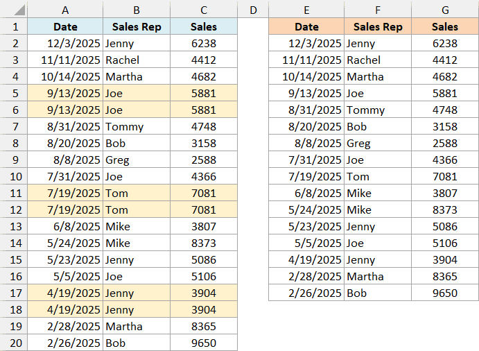
Suppose you have a dataset as shown below (this is the Unique Records sheet in the example file), and you want the unique records in columns E to G.

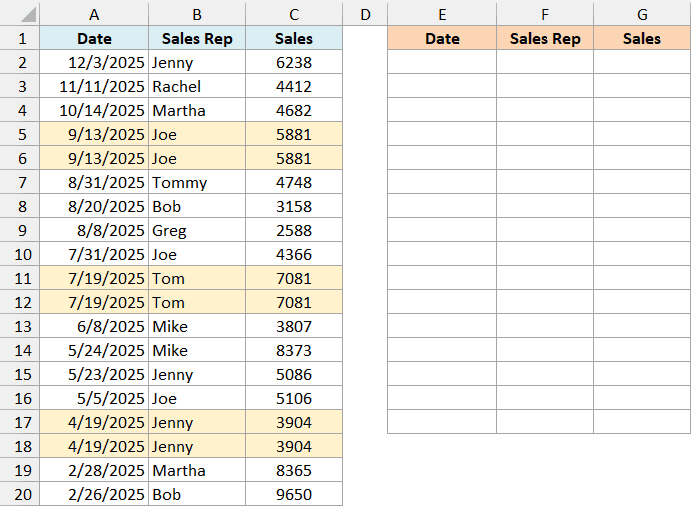
As you can see, there are duplicate records in this data set (highlighted in yellow). These could be due to an error in data entry or result of data compilation.

In such a case, you can use Excel Advanced Filter tool to quickly get a list of all the unique records in a different location (so that your original data remains intact).

Here are the steps to get all the unique records:

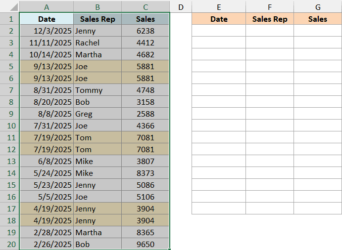
1. Select the entire data set (including the headers), which is A1:C20 in this example.

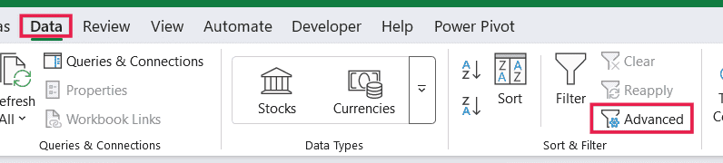
2. Click the Data tab, then click Advanced in the Sort & Filter group. (You can also use the keyboard shortcut Alt + A + Q on Windows). This will open the Advanced Filter dialog box.

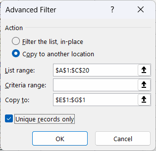
3. In the Advanced Filter dialog box, use the following details:
   • Action: Select the ‘Copy to another location’ option. This will allow you to specify the location where you can get the list of unique records.
   • List range: Make sure it refers to the dataset from which you want to find unique records (A1:C20). Also, make sure headers in the data set are included.
   • Criteria range: Leave this empty.
   • Copy to: Specify the cell address where you want to get the list of unique records (E1:G1, which has a copy of the headers).
   • Unique records only: Check this option.

4. Click OK.

This will instantly give you a list of all the unique records. In this example, the 19 records come down to 16.

A record counts as a duplicate only when every column matches. That’s why Joe still appears more than once in the result (his 4 rows become 3, because only one of them was an exact repeat).

Important: When you are using Advanced Filter to get the unique list, make sure you have also selected the header. If you don’t, it would consider the first record as the header.

If you want each name listed only once, you can get the unique values from just one column.

Use only that column as the List range (B1:B20 for the Sales Rep names) and an empty cell such as I1 as the Copy to cell, and you get the 9 names.

Filter on Multiple Criteria with Excel Advanced Filter

Getting unique records is one of the many things you can do with Excel advanced filter.

Its primary utility lies in its ability to allow using complex criteria for filtering data.

Here is what I mean by complex criteria.

Suppose you have a dataset as shown below (this is the AND – US Over 5000 sheet in the example file) and you want to quickly get all the records where the sales are greater than 5000 and the region is the US.

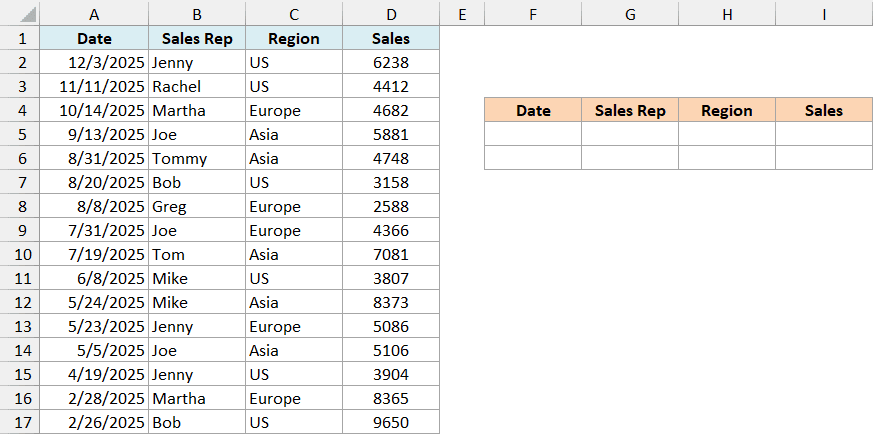
Here is how you can use Excel Advanced Filter to filter the records based on the specified criteria:

1. The first step when using Excel Advanced Filter with complex criteria is to specify the criteria. To do this, copy the headers and paste them somewhere in the worksheet (F1:I1 in this example).

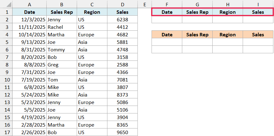
Remember, the headers in the criteria should be exactly the same as that in the data set. If a header has a typo, Excel can’t match the condition under it and you get no records at all.

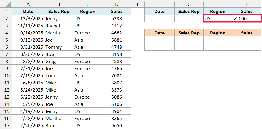
2. Specify the criteria for which you want to filter the data. In this example, since we want to get all the records for the US with sales more than 5000, enter ‘US’ in the cell below Region and >5000 in the cell below Sales. This would now be used as an input in Advanced Filter to get the filtered data (as shown in the next steps).

3. Select the entire data set (including the headers).

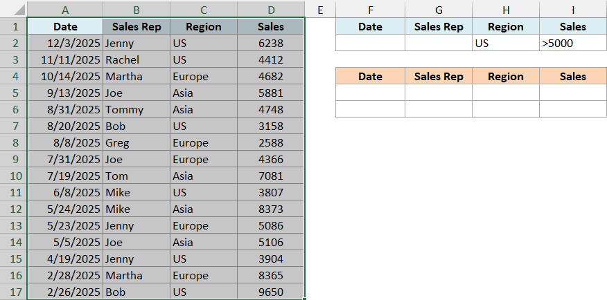
4. Click the Data tab, then click Advanced in the Sort & Filter group. This will open the Advanced Filter dialog box.

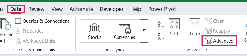
5. In the Advanced Filter dialog box, use the following details:
   • Action: Select the ‘Copy to another location’ option. This will allow you to specify the location where you can get the filtered records.
   • List range: Make sure it refers to the dataset you want to filter (A1:D17). Also, make sure headers in the data set are included.
   • Criteria range: Specify the criteria we constructed in the steps above. In this example, it would be F1:I2.
   • Copy to: Specify the cell address where you want to get the filtered records. In this example, it’s F4:I4, which has a copy of the headers. If you don’t have the headers in place, you can enter a single empty cell instead, and Excel adds all the headers for you.
   • Unique records only: Leave this unchecked. If you check it, any record that appears twice in your data shows up only once in the result.

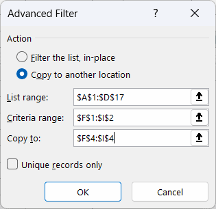
Important: Include only the rows that have criteria in the Criteria range. If it also includes a blank row (F1:I3 here), Excel reads that blank row as no condition at all and gives you every record.

6. Click OK.

This would instantly give you all the records where the region is the US and the sales are more than 5000.

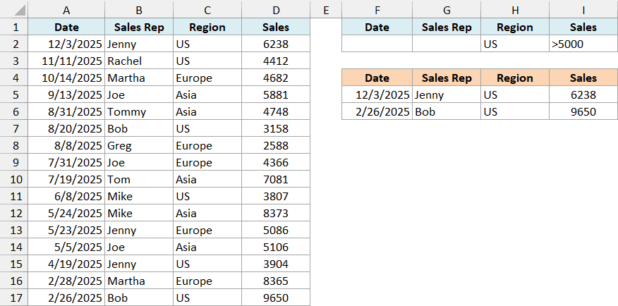
Note that the result is a snapshot. If you change a criterion or the data later, the copied records stay as they are, so you need to run the Advanced Filter again.

Advanced filtering cannot be undone when copied to other locations, so double-check the Copy to range before you click OK.

The above example is a case where the filtering is done based on two criteria (US and sales greater than 5000).

Excel Advanced filter allows you to create many different combinations of criteria.

Here are some examples of how you can construct these filters.

Using the AND Criteria in Advanced Filter

When you want to use AND criteria, you need to specify it below the header, with all the conditions in the same row.

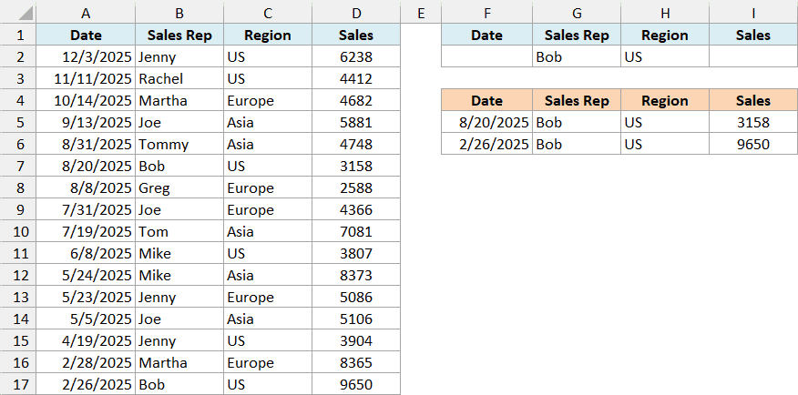
For example, to filter records when the region is the US AND the sales rep is Bob, enter Bob below Sales Rep and US below Region (this is the AND – US and Bob sheet in the example file).

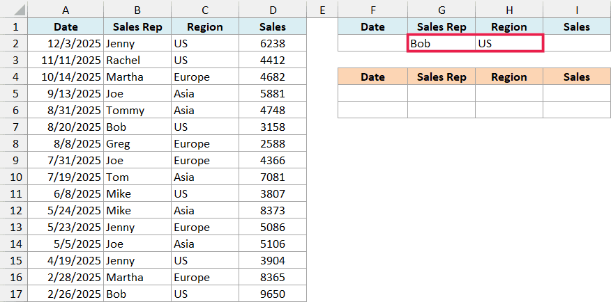
In the Advanced Filter dialog box, use A1:D17 as the List range, F1:I2 as the Criteria range, and F4:I4 as the Copy to range. This gives you the two records for Bob in the US.

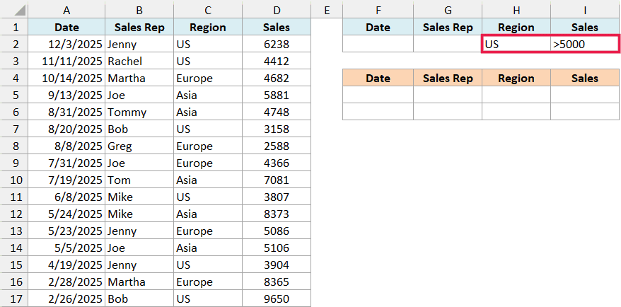
To filter records when the region is the US AND the sales value is greater than 5000, enter US below Region and >5000 below Sales. This is the example we did above (the AND – US Over 5000 sheet in the example file).

To filter records when the region is the US AND the sales are recorded after 31-Mar-2025, enter >31-Mar-2025 below Date and US below Region (this is the AND – US After Date sheet in the example file).

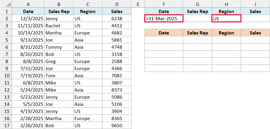
With the same three ranges in the dialog box, you get the five US records after that date.

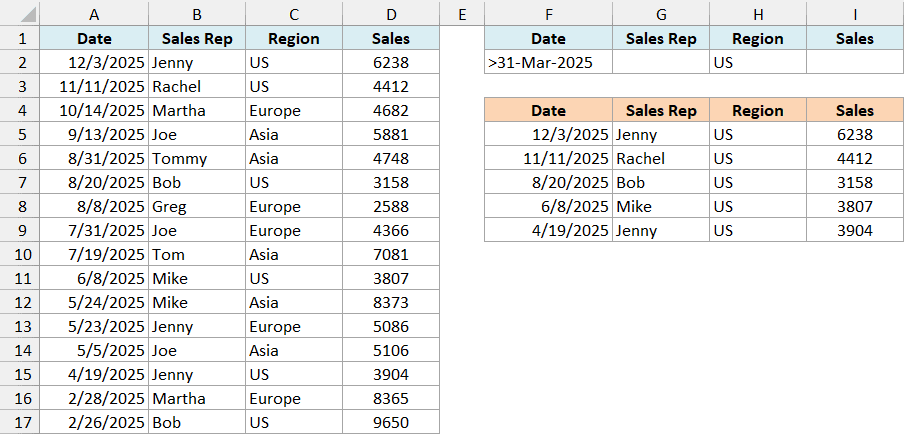
Excel reads a date in a criteria cell using your computer’s regional settings. So on a PC set to US dates, >31-03-2025 returns nothing, because Excel can’t read 31-03 as a date there.

That’s why I’ve spelled out the month here. If that doesn’t work on your PC, enter =">"&DATE(2025,3,31) in the cell instead, because the DATE function gives Excel the date without any format to guess at.

Using the OR Criteria in Advanced Filter

When you want to use OR criteria, you need to specify the criteria in different rows. They can be in the same column or in different columns.

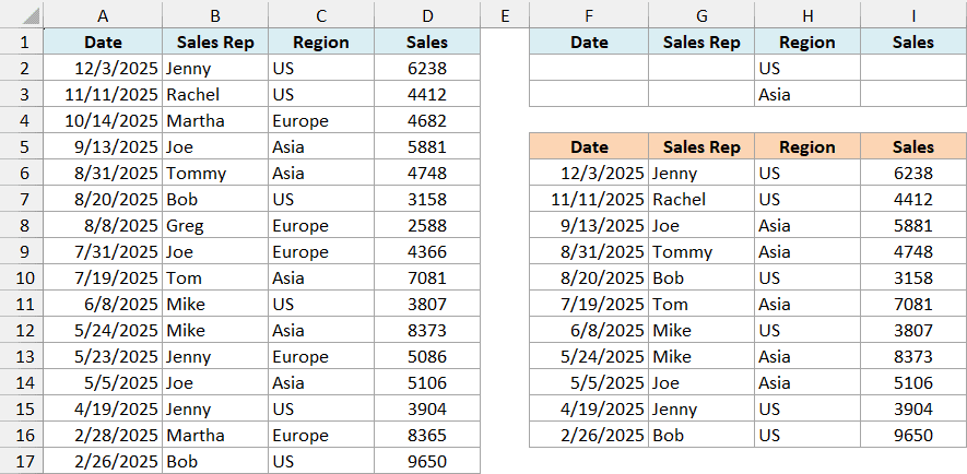
For example, to filter records when the region is the US OR the region is Asia, enter US and Asia one below the other below Region (this is the OR – US or Asia sheet in the example file).

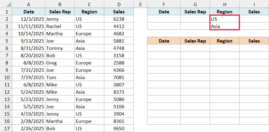
Since the criteria now take up two rows, use F1:I3 as the Criteria range and F5:I5 as the Copy to range, with A1:D17 as the List range. This gives you all 11 records for the US and Asia.

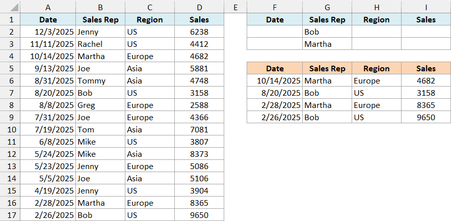
To filter records when the Sales rep is Bob OR Martha, enter both names one below the other below Sales Rep (this is the OR – Bob or Martha sheet in the example file).

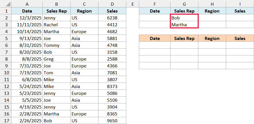
With the same three ranges in the dialog box, you get the four records for Bob and Martha.

The conditions don’t have to be in the same column.

To filter records when the region is Asia OR the sales are greater than 8000, enter Asia below Region in the first row and >8000 below Sales in the second row (this is the OR – Asia or Over 8000 sheet in the example file).

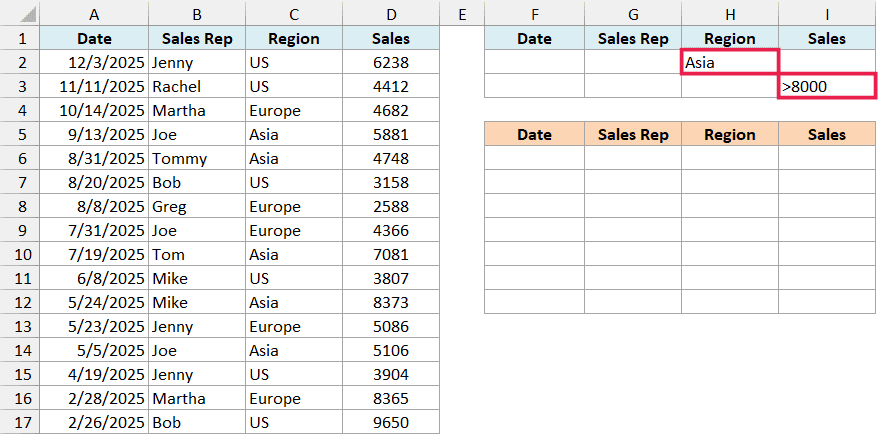
A record has to match only one of the two rows, so with the same three ranges you get seven records. That includes the Martha and Bob records from outside Asia, because their sales are above 8000.

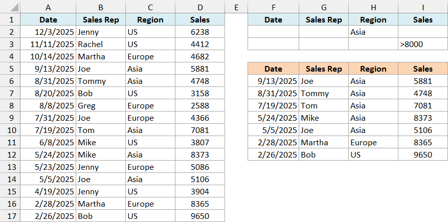
Pro Tip: By now, you must have realized that when we have the criteria in the same row, it is an AND criteria, and when we have it in different rows, it is an OR criteria.

Combine AND and OR Criteria in Advanced Filter

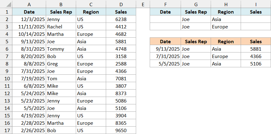
You can use both in the same filter. Suppose you want the records where the sales rep is Joe and the region is either Asia or Europe.

To do this, enter Joe and Asia in the first criteria row, and Joe and Europe in the second row (this is the AND OR – Joe Asia or Europe sheet in the example file).

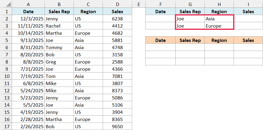
Make sure Joe is in both rows. If you enter it only in the first row, the second row asks for every Europe record, no matter who the sales rep is.

Use A1:D17 as the List range, F1:I3 as the Criteria range, and F5:I5 as the Copy to range. This gives you Joe’s three records.

Filter Values Between Two Numbers

To filter a range of values, you need two conditions on the same column, which means the same header has to appear twice in the criteria.

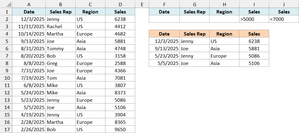
Below is the sales dataset (this is the Between 5000 and 7000 sheet in the example file), and I want the records with sales between 5000 and 7000. The criteria have two Sales headers, with >5000 below one and <7000 below the other.

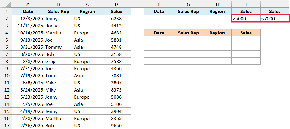
Both conditions are in the same row, so a record has to meet both. Use A1:D17 as the List range, F1:J2 as the Criteria range, and F4:I4 as the Copy to range to get the four records in that range.

Filter for an Exact Match in Advanced Filter

When you enter text as a criterion, Advanced Filter looks for any value that begins with that text, and it ignores upper and lower case. This is easy to miss, because most of the time the result looks right.

Below is a dataset where I have entered Tom below Sales Rep, and I want the records for Tom in columns F to I (this is the Text – Starts With Tom sheet in the example file).

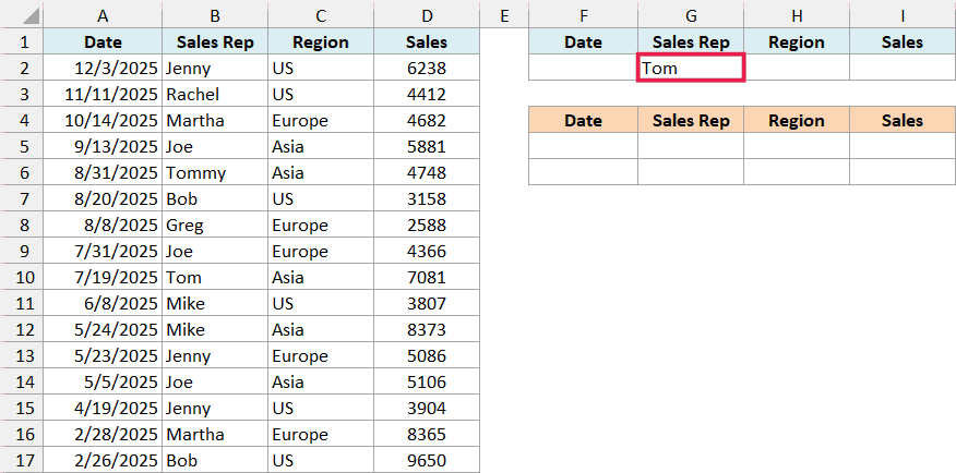
Use A1:D17 as the List range, F1:I2 as the Criteria range, and F4:I4 as the Copy to range. You get two records, because Tommy also begins with Tom.

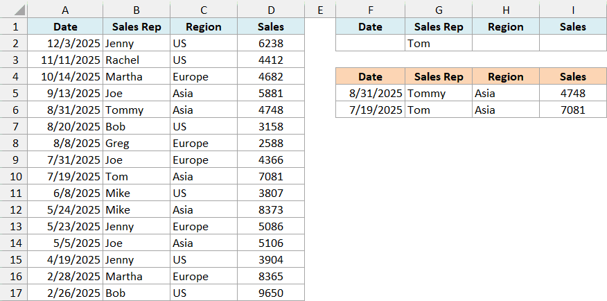
To get only Tom, enter the below formula in the cell below Sales Rep (this is the Text – Exactly Tom sheet in the example file):

="=Tom"

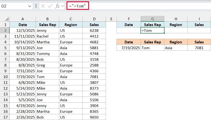
With the same three ranges, you now get only the one record for Tom. The equal sign in what the cell displays (=Tom) is what tells Advanced Filter to match the whole value and not just the beginning.

Don’t type =Tom directly though, because Excel would treat it as a formula and give you a #NAME? error. Also note that this still ignores case, so ="=tom" gives you the same record.

Using Wildcard Characters in Advanced Filter

Excel Advanced Filter also allows the usage of wildcard characters while constructing the criteria.

There are three wildcard characters in Excel:

1. * (asterisk): It represents any number of characters. For example, ex* could mean excel, excels, example, expert, etc.
2. ? (question mark): It represents one single character. For example, Tr?mp could mean Trump or Tramp.
3. ~ (tilde): It is used to identify a wildcard character (~, *, ?) in the text.

Now let’s see how we can use these wildcard characters to do some advanced filtering in Excel.

To filter records where the sales rep name starts from J, enter J* below Sales Rep (this is the Wildcard – Starts With J sheet in the example file).

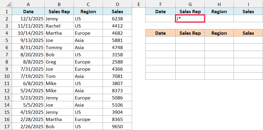
Note that * represent any number of characters. So any rep with the name starting with J would be filtered with these criteria.

Use A1:D17 as the List range, F1:I2 as the Criteria range, and F4:I4 as the Copy to range. This gives you the six records for Jenny and Joe.

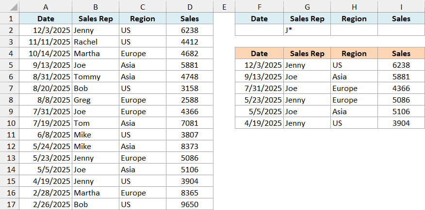
Since text criteria already look at the start of a value, a plain J would give you the same six records here. Wildcards get more useful when the text you want isn’t at the start.

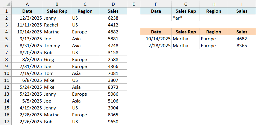
For example, to filter records where the name has “ar” anywhere in it, enter *ar* below Sales Rep (this is the Wildcard – Contains ar sheet in the example file).

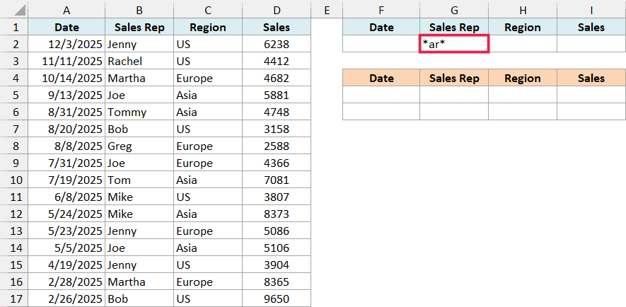
With the same three ranges, you get the two records for Martha.

Similarly, you can use the other two wildcard characters as well.

The tilde is for values that really have a wildcard character in them. For example, if a sales rep was entered as Joe*, then Joe~* finds only that value, while Joe* would find every name starting with Joe.

Just remember that a criterion like ?o? still works as a begins-with match, so it also picks up Tommy. To limit it to three-letter names like Bob, Joe, and Tom, enter it as ="=?o?".

Use a Formula as the Criteria in Advanced Filter

Some conditions can’t be typed as a simple value, such as sales above the average. For these, you can use a formula that returns TRUE or FALSE as the criteria.

There are three rules for this, and getting any of them wrong gives you the wrong records:

• The label above the formula can’t be a header from your dataset. Use your own text (or leave it blank). With a real header such as Sales above the formula, you get no records.
• Refer to the first data row with a relative reference, such as D2 for the first sales value. Excel moves this reference down as it checks each record. If you lock it (D$2), Excel checks the same cell every time, so you get either every record or none of them.
• Make every other reference absolute, such as $D$2:$D$17 for the whole Sales column. Otherwise, this range would shift down along with D2, and the formula would stop looking at the full column.

Below is the sales dataset (this is the Formula – Above Average sheet in the example file), and I want the records with above-average sales in columns H to K.

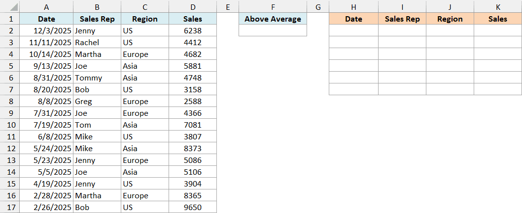
Here is the formula to enter in F2, with Above Average as the label in F1:

=D2>AVERAGE($D$2:$D$17)

Use A1:D17 as the List range, F1:F2 as the Criteria range, and H1:K1 as the Copy to range. This gives you the six records with sales above the average of about 5465.

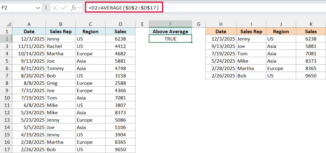
F2 shows TRUE because it only has the result for the first record (6238 is above the average). Excel runs the formula for every record when you click OK.

If you add more rows to your data, extend $D$2:$D$17 to cover them.

You can also use this to filter against a list.

Below I have a list of sales reps in H2:H3 (this is the Formula – Reps on a List sheet in the example file), and I want all the records for these reps in columns J to M.

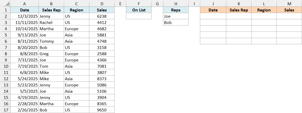
Here is the formula to enter in F2, with On List as the label in F1:

=COUNTIF($H$2:$H$3,B2)>0

Use A1:D17 as the List range, F1:F2 as the Criteria range, and J1:M1 as the Copy to range. This gives you the five records for Joe and Bob.

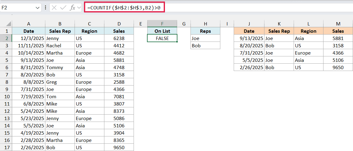
The COUNTIF function checks whether the sales rep in each record appears in the list. F2 shows FALSE because the first record is for Jenny, who isn’t on the list, and that’s fine.

If you add a name to the list, extend $H$2:$H$3 to include it. Also note that the COUNTIF function ignores case, so joe on the list would also match Joe.

Copy Only the Columns You Want with Advanced Filter

When your Copy to range has all the headers, you get all the columns. If you only need some of them, type just those headers where you want the result and use them as the Copy to range.

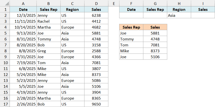
Below is the sales dataset (this is the Chosen Columns sheet in the example file), and I want only the Sales Rep and Sales columns for the Asia records in columns F and G.

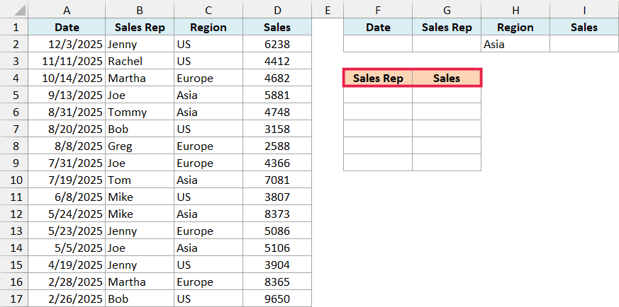
Use A1:D17 as the List range, F1:I2 as the Criteria range, and F4:G4 as the Copy to range. This gives you the two columns for the five Asia records.

Copy Advanced Filter Results to Another Sheet

You can also get the result on a different sheet from your data, but you need to start from the sheet where you want the result.

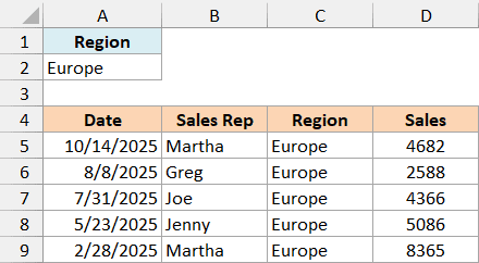
Below is a sales dataset on the Sales Data sheet in the example file, and I want the Europe records on the Filtered Sales sheet.

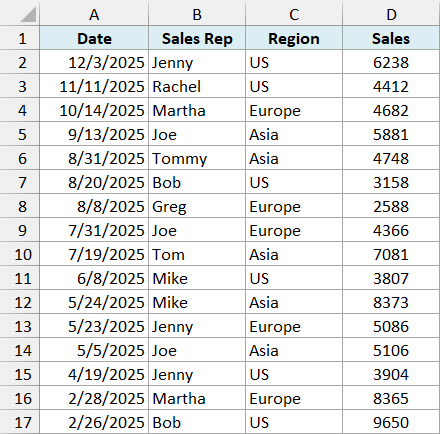
Here are the steps to do this:

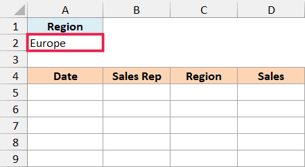
1. Go to the Filtered Sales sheet, which has the criteria in A1:A2.

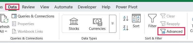
2. Click the Data tab, then click Advanced in the Sort & Filter group.

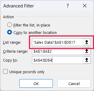
3. In the Advanced Filter dialog box, select ‘Copy to another location’, then click in the List range box and select A1:D17 on the Sales Data sheet. Use A1:A2 as the Criteria range and A4:D4 as the Copy to range.

4. Click OK.

This gives you the five Europe records on the Filtered Sales sheet, while your data stays where it is.

Important: If you start from the Sales Data sheet and point Copy to at another sheet, Excel stops you with the error “You can only copy filtered data to the active sheet”. Close the dialog box and start again from the destination sheet.

Filter the Data in Place with Advanced Filter

You don’t have to copy the result anywhere. If you want to hide the rows that don’t match, like the regular filter does, you can filter the data in place.

Below is the sales dataset (this is the AND – US Over 5000 sheet in the example file), and I want to see only the US records with sales over 5000 in the dataset itself.

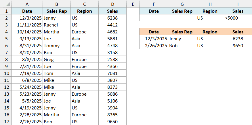
In the Advanced Filter dialog box, select ‘Filter the list, in-place’, use A1:D17 as the List range and F1:I2 as the Criteria range, and click OK. Excel hides the 14 rows that don’t match.

Excel hides the entire row, so anything next to your data on those rows gets hidden too. In this sheet, that includes the records copied to F4:I6 in the earlier example.

To get all the rows back, click the Data tab and then click Clear in the Sort & Filter group.

Advanced Filter vs the FILTER Function

In case you’re using Excel 2021 or later, or Microsoft 365, you should check out the FILTER function. It can do a lot of things that advanced filter can do with a simple formula.

Below is the same sales dataset (this is the FILTER Function sheet in the example file), and I want the US records with sales over 5000 in columns F to I.

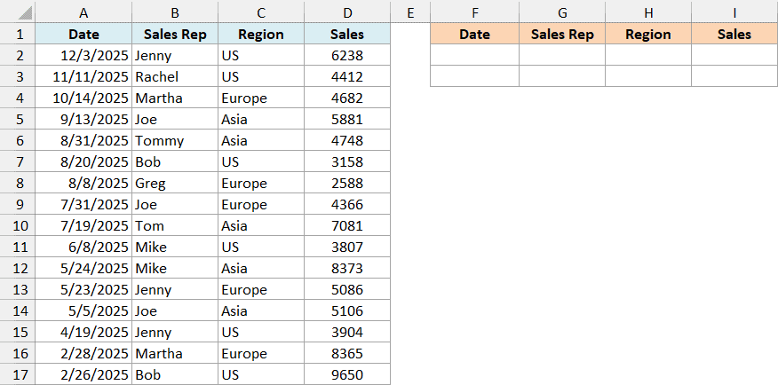
Here is the formula to enter in F2:

=FILTER(A2:D17,(C2:C17="US")*(D2:D17>5000))

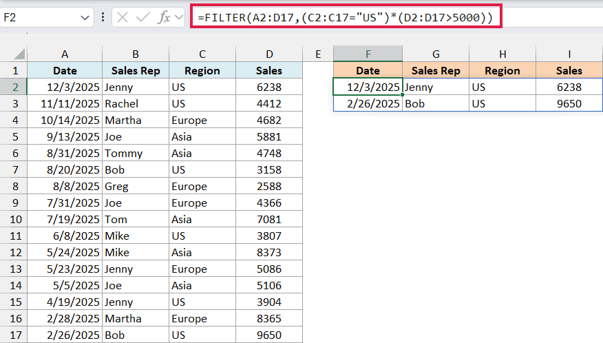
This gives you the same two records as the Advanced Filter example above, and the result spills down on its own. Multiplying the two conditions means a record has to meet both.

The big difference is that the FILTER function updates when your data changes, while the Advanced Filter result stays as it was until you run it again.

So the Advanced Filter is the one to use on older Excel versions, or when you want a copy that doesn’t change.

If no record matches, this formula gives a #CALC! error. The FILTER function has an optional third argument to show your own text in that case.

So these are some of the ways you can use the Excel Advanced Filter. If your result ever looks wrong, check the Criteria range first, because a blank row or a misspelled header changes what you get.

I hope you found this Excel tutorial useful.

Other Excel Articles You May Also Like:

• Dynamic Excel Filter – Extract Data as you Type.
• Filtering Cells with Bold Font Formatting.
• How to Filter Cells that have Duplicate Text Strings (Words) in it.
• How to Filter Data in a Pivot Table in Excel
• MS Guide for Advanced Filter in Excel.
• How to Compare Two Columns in Excel.
• Excel VBA Autofilter
• 20 Advanced Excel Functions and Formulas (for Excel Pros)
• How to Create a Drop Down Filter in Excel (Extract Data Based on Selection)
• Delete Rows Based on a Cell Value (or Condition) in Excel