
A lot of Excel functionalities are also available to be used in VBA – and the Autofilter method is one such functionality.
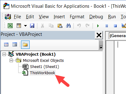
If you have a dataset and you want to filter it using a criterion, you can easily do it using the Filter option in the Data ribbon.![]()
And if you want a more advanced version of it, there is an advanced filter in Excel as well.
Then Why Even Use the AutoFilter in VBA?
If you just need to filter data and do some basic stuff, I would recommend stick to the inbuilt Filter functionality that Excel interface offers.
You should use VBA Autofilter when you want to filter the data as a part of your automation (or if it helps you save time by making it faster to filter the data).
For example, suppose you want to quickly filter the data based on a drop-down selection, and then copy this filtered data into a new worksheet.
While this can be done using the inbuilt filter functionality along with some copy-paste, it can take you a lot of time to do this manually.
In such a scenario, using VBA Autofilter can speed things up and save time.
Note: I will cover this example (on filtering data based on a drop-down selection and copying into a new sheet) later in this tutorial.
Excel VBA Autofilter Syntax
Expression. AutoFilter( _Field_ , _Criteria1_ , _Operator_ , _Criteria2_ , _VisibleDropDown_ )
- Expression: This is the range on which you want to apply the auto filter.
- Field: [Optional argument] This is the column number that you want to filter. This is counted from the left in the dataset. So if you want to filter data based on the second column, this value would be 2.
- Criteria1: [Optional argument] This is the criteria based on which you want to filter the dataset.
- Operator: [Optional argument] In case you’re using criteria 2 as well, you can combine these two criteria based on the Operator. The following operators are available for use: xlAnd, xlOr, xlBottom10Items, xlTop10Items, xlBottom10Percent, xlTop10Percent, xlFilterCellColor, xlFilterDynamic, xlFilterFontColor, xlFilterIcon, xlFilterValues
- Criteria2: [Optional argument] This is the second criteria on which you can filter the dataset.
- VisibleDropDown: [Optional argument] You can specify whether you want the filter drop-down icon to appear in the filtered columns or not. This argument can be TRUE or FALSE.
Apart from Expression, all the other arguments are optional.
In case you don’t use any argument, it would simply apply or remove the filter icons to the columns.
Sub FilterRows()
Worksheets("Filter Data").Range("A1").AutoFilter
End Sub
The above code would simply apply the Autofilter method to the columns (or if it’s already applied, it will remove it).
This simply means that if you can not see the filter icons in the column headers, you will start seeing it when this above code is executed, and if you can see it, then it will be removed.
In case you have any filtered data, it will remove the filters and show you the full dataset.
Now let’s see some examples of using Excel VBA Autofilter that will make it’s usage clear.
Example: Filtering Data based on a Text condition
Suppose you have a dataset as shown below and you want to filter it based on the ‘Item’ column.
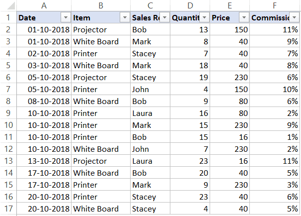
The below code would filter all the rows where the item is ‘Printer’.
Sub FilterRows()
Worksheets("Sheet1").Range("A1").AutoFilter Field:=2, Criteria1:="Printer"
End Sub
The above code refers to Sheet1 and within it, it refers to A1 (which is a cell in the dataset).
Note that here we have used Field:=2, as the item column is the second column in our dataset from the left.
Now if you’re thinking – why do I need to do this using a VBA code. This can easily be done using inbuilt filter functionality. You’re right! If this is all you want to do, better used the inbuilt Filter functionality. But as you read the remaining tutorial, you’ll see that this can be combined with some extra code to create powerful automation.
But before I show you those, let me first cover a few examples to show you what all the AutoFilter method can do.
Click here to download the example file and follow along.
Example: Multiple Criteria (AND/OR) in the Same Column
Suppose I have the same dataset, and this time I want to filter all the records where the item is either ‘Printer’ or ‘Projector’.
The below code would do this:
Sub FilterRowsOR()
Worksheets("Sheet1").Range("A1").AutoFilter Field:=2, Criteria1:="Printer", Operator:=xlOr, Criteria2:="Projector"
End Sub
Note that here I have used the xlOR operator.
This tells VBA to use both the criteria and filter the data if any of the two criteria are met.
Similarly, you can also use the AND criteria.
For example, if you want to filter all the records where the quantity is more than 10 but less than 20, you can use the below code:
Sub FilterRowsAND()
Worksheets("Sheet1").Range("A1").AutoFilter Field:=4, Criteria1:=">10", _
    Operator:=xlAnd, Criteria2:="<20"
End Sub
Example: Multiple Criteria With Different Columns
Suppose you have the following dataset.
With Autofilter, you can filter multiple columns at the same time.
For example, if you want to filter all the records where the item is ‘Printer’ and the Sales Rep is ‘Mark’, you can use the below code:
Sub FilterRows()
With Worksheets("Sheet1").Range("A1")
.AutoFilter field:=2, Criteria1:="Printer"
.AutoFilter field:=3, Criteria1:="Mark"
End With
End Sub
Example: Filter Top 10 Records Using the AutoFilter Method
Suppose you have the below dataset.
Below is the code that will give you the top 10 records (based on the quantity column):
Sub FilterRowsTop10()
ActiveSheet.Range("A1").AutoFilter Field:=4, Criteria1:="10", Operator:=xlTop10Items
End Sub
In the above code, I have used ActiveSheet. You can use the sheet name if you want.
Note that in this example, if you want to get the top 5 items, just change the number in Criteria1:=”10″ from 10 to 5.
So for top 5 items, the code would be:
Sub FilterRowsTop5()
ActiveSheet.Range("A1").AutoFilter Field:=4, Criteria1:="5", Operator:=xlTop10Items
End Sub
It may look weird, but no matter how many top items you want, the Operator value always remains xlTop10Items.
Similarly, the below code would give you the bottom 10 items:
Sub FilterRowsBottom10()
ActiveSheet.Range("A1").AutoFilter Field:=4, Criteria1:="10", Operator:=xlBottom10Items
End Sub
And if you want the bottom 5 items, change the number in Criteria1:=”10″ from 10 to 5.
Example: Filter Top 10 Percent Using the AutoFilter Method
Suppose you have the same data set (as used in the previous examples).
Below is the code that will give you the top 10 percent records (based on the quantity column):
Sub FilterRowsTop10()
ActiveSheet.Range("A1").AutoFilter Field:=4, Criteria1:="10", Operator:=xlTop10Percent
End Sub
In our dataset, since we have 20 records, it will return the top 2 records (which is 10% of the total records).
Example: Using Wildcard Characters in Autofilter
Suppose you have a dataset as shown below:
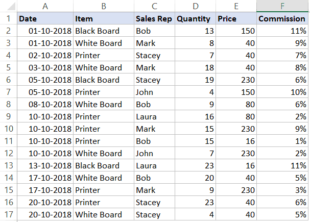
If you want to filter all the rows where the item name contains the word ‘Board’, you can use the below code:
Sub FilterRowsWildcard()
Worksheets("Sheet1").Range("A1").AutoFilter Field:=2, Criteria1:="*Board*"
End Sub
In the above code, I have used the wildcard character * (asterisk) before and after the word ‘Board’ (which is the criteria).
An asterisk can represent any number of characters. So this would filter any item that has the word ‘board’ in it.
Example: Copy Filtered Rows into a New Sheet
If you want to not only filter the records based on criteria but also copy the filtered rows, you can use the below macro.
It copies the filtered rows, adds a new worksheet, and then pastes these copied rows into the new sheet.
Sub CopyFilteredRows()
Dim rng As Range
Dim ws As Worksheet
If Worksheets("Sheet1").AutoFilterMode = False Then
MsgBox "There are no filtered rows"
Exit Sub
End If
Set rng = Worksheets("Sheet1").AutoFilter.Range
Set ws = Worksheets.Add
rng.Copy Range("A1")
End Sub
The above code would check if there are any filtered rows in Sheet1 or not.
If there are no filtered rows, it will show a message box stating that.
And if there are filtered rows, it will copy those, insert a new worksheet, and paste these rows on that newly inserted worksheet.
Example: Filter Data based on a Cell Value
Using Autofilter in VBA along with a drop-down list, you can create a functionality where as soon as you select an item from the drop-down, all the records for that item are filtered.
Something as shown below:
 Click here to download the example file and follow along.
This type of construct can be useful when you want to quickly filter data and then use it further in your work.
Below is the code that will do this:
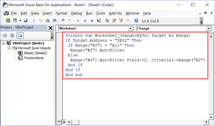
Private Sub Worksheet_Change(ByVal Target As Range)
If Target.Address = "$B$2" Then
 If Range("B2") = "All" Then
  Range("A5").AutoFilter
 Else
  Range("A5").AutoFilter Field:=2, Criteria1:=Range("B2")
 End If
End If
End Sub
This is a worksheet event code, which gets executed only when there is a change in the worksheet and the target cell is B2 (where we have the drop-down).
Also, an If Then Else condition is used to check if the user has selected ‘All’ from the drop down. If All is selected, the entire data set is shown.
This code is NOT placed in a module.
Instead, it needs to be placed in the backend of the worksheet that has this data.
Here are the steps to put this code in the worksheet code window:
- Open the VB Editor (keyboard shortcut – ALT + F11).
- In the Project Explorer pane, double-click on the Worksheet name in which you want this filtering functionality.
- In the worksheet code window, copy and paste the above code.
- Close the VB Editor.
Now when you use the drop-down list, it will automatically filter the data.
This is a worksheet event code, which gets executed only when there is a change in the worksheet and the target cell is B2 (where we have the drop-down).
Also, an If Then Else condition is used to check if the user has selected ‘All’ from the drop down. If All is selected, the entire data set is shown.
Turn Excel AutoFilter ON/OFF using VBA
When applying Autofilter to a range of cells, there may already be some filters in place.
You can use the below code turn off any pre-applied auto filters:
Sub TurnOFFAutoFilter()
  Worksheets("Sheet1").AutoFilterMode = False
End Sub
This code checks the entire sheets and removes any filters that have been applied.
If you don’t want to turn off filters from the entire sheet but only from a specific dataset, use the below code:
Sub TurnOFFAutoFilter()
  If Worksheets("Sheet1").Range("A1").AutoFilter Then
    Worksheets("Sheet1").Range("A1").AutoFilter
  End If
End Sub
The above code checks whether there are already filters in place or not.
If filters are already applied, it removes it, else it does nothing.
Similarly, if you want to turn on AutoFilter, use the below code:
Sub TurnOnAutoFilter()
  If Not Worksheets("Sheet1").Range("A4").AutoFilter Then
    Worksheets("Sheet1").Range("A4").AutoFilter
  End If
End Sub
Check if AutoFilter is Already Applied
If you have a sheet with multiple datasets and you want to make sure you know that there are no filters already in place, you can use the below code.
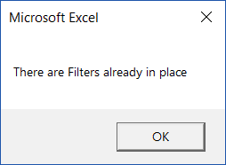
Sub CheckforFilters()
If ActiveSheet.AutoFilterMode = True Then
MsgBox "There are Filters already in place"
Else
MsgBox "There are no filters"
End If
End Sub
This code uses a message box function that displays a message ‘There are Filters already in place’ when it finds filters on the sheet, else it shows ‘There are no filters’.
Show All Data
If you have filters applied to the dataset and you want to show all the data, use the below code:
Sub ShowAllData()
If ActiveSheet.FilterMode Then ActiveSheet.ShowAllData
End Sub
The above code checks whether the FilterMode is TRUE or FALSE.
If it’s true, it means a filter has been applied and it uses the ShowAllData method to show all the data.
Note that this does not remove the filters. The filter icons are still available to be used.
Using AutoFilter on Protected Sheets
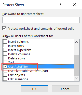
By default, when you protect a sheet, the filters won’t work.
In case you already have filters in place, you can enable AutoFilter to make sure it works even on protected sheets.
To do this, check the Use Autofilter option while protecting the sheet.
While this works when you already have filters in place, in case you try to add Autofilters using a VBA code, it won’t work.
Since the sheet is protected, it wouldn’t allow any macro to run and make changes to the Autofilter.
So you need to use a code to protect the worksheet and make sure auto filters are enabled in it.
This can be useful when you have created a dynamic filter (something I covered in the example – ‘Filter Data based on a Cell Value’).
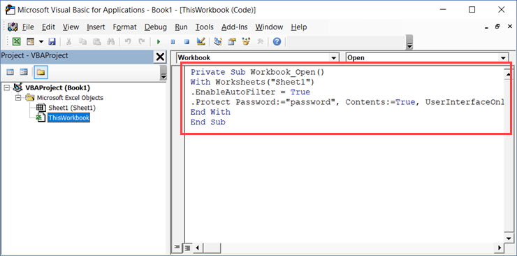
Below is the code that will protect the sheet, but at the same time, allow you to use Filters as well as VBA macros in it.
Private Sub Workbook_Open()
With Worksheets("Sheet1")
.EnableAutoFilter = True
.Protect Password:="password", Contents:=True, UserInterfaceOnly:=True
End With
End Sub
This code needs to be placed in ThisWorkbook code window.
Here are the steps to put the code in ThisWorkbook code window:
- Open the VB Editor (keyboard shortcut – ALT + F11).
- In the Project Explorer pane, double-click on the ThisWorkbook object.
- In the code window that opens, copy and paste the above code.
As soon as you open the workbook and enable macros, it will run the macro automatically and protect Sheet1.
However, before doing that, it will specify ‘EnableAutoFilter = True’, which means that the filters would work in the protected sheet as well.
Also, it sets the ‘UserInterfaceOnly’ argument to ‘True’. This means that while the worksheet is protected, the VBA macros code would continue to work.
You May Also Like the Following VBA Tutorials:


your site is very helpfull to me!
Is it possible to make the Field number dynamic?
In my case the column number changes when a new date is created.
The column was for instance 10 and now 11 or higher.
Hi how would you autofilter alphanumeric values in a column, examples are
column 1 has A3 Cell contains the value-Joe 2516, A4 has value- Jenny2517 Cell A5 has 2875Ani, Cell A6 has 1092-Naomi
Is it possible to get some al the values out column 3 after filtering on a other sheet
This is truly a remarkable website for Excel VBA tutorials and it has helped me enormously in trying to automate searches and filters in my personal book catalogue. But of course I have a question 🙂 which I hope will provide a tutorial for us all to appreciate. My book catalogue is an Excel worksheet which I convertd to an Excel Table to which I have applied a top row of buttons that apply filters on column 3 with each button filtering book types like Travel, History, Psychology, Psychodratic Bodywork, etc. I would like to use VBA to total and display the result of each search?
Hi, I want to know if its possible to filter by a week number, as example having week number in a cell.
Thanks.
it’s a great macro. keep it ahead
Something I’m not clear about. I always see these filters with 1 or 2 criteria. Is it possible to have 3+ criteria, e.g.
With Worksheets(“Sheet1”).Range(“A1″)
.AutoFilter field:=2, Criteria1:=”Printer”
.AutoFilter field:=3, Criteria1:=”Mark”
.AutoFilter field:=5, Criteria1:=”Fax”
.AutoFilter field:=9, Criteria1:=<15
End With
Also, is it possible to have several .AutoFilters on the same field without using Criteria2, i.e.
With Worksheets("Sheet1").Range("A1")
.AutoFilter field:=2, Criteria1:="Printer”
.AutoFilter field:=2, Criteria1:=”Fax”
.AutoFilter field:=2, Criteria1:=”Copier”
.AutoFilter field:=9, Criteria1:=<15
End With
I have a case where I want to filter out text that matches any of several long boilerplate strings.
Also, can Criteria1 (or 2) use a UDF?
yes it’s Possible
this will let you add more than 2 Criteria in the same Field
.AutoFilter 2, Criteria1:=Array(“Printer”, ”Fax”, ”Copier”), Operator:=xlFilterValues
I need to filter the data for rows that match a value entered in another cell. You have an example using a drop down, but I don’t want to use a drop down. Techs would use the shared file, enter their tech number and see their work listed in the spreadsheet. I don’t want them being able to pull up other tech’s data using a drop down.
Thank you, Sumit. This tutorial is very clear and easy to follow.
Thanks Bill.. Glad you found it useful!
Very nice tutorial, but why did you protect the example file?
If you share an example file, usually it’s because you want people to see how it was done.
I have no use for a locked example file.
Ok, I didn’t read through the end, my bad!
How do you change the code to filter for all items but not 1 specific (or 2 for that matter) i.e. if i tried to select all items apart from ‘Opening Balance’ I tried the below but it wont work
Worksheets(“Sheet1”).Range(“A1″).AutoFilter Field:=2, Criteria1:=”Opening Balance”
Is there a way to instruct VBA to select all items but not (different than) something?
I want to use filter option for a group of excel worksheets. The sheets contain same column heading e.g. Name, Address, post code, phone number etc. I want to use filtering option to be applied for all sheets at a time. Filtering one by one sheet is time consuming. So please help me on this point.
sipppp, tanks so much
Hi the above example really worth. But we need how to convert DAT. File into an excel file from folder, from there how to apply filter criteria and the output saved different workbook
Tutorial is excellent , wanted to know how to go to last cell of the filtered column in macro as we will never know where my last cell is , so how to get to that cell for further work
very good tutorial
Amazing, thank you very much, this is very helpful article.
In case several options need to be chosen from a column (not just one, or two), ARRAY could be used. Would it be possible to add this exemple into your article ?
That’s what I’m looking for as well. Two criteria is often just not enough, an array would be perfect.
Simply fantastic work, very well done, Sir !