Filter By Color in Excel

Watch Video – Filter by Color in Excel (Cell Color or Font Color)

Filtering your data is a common task for many Excel users as a part of their daily work.

Excel already has a well-developed filter functionality that allows you to filter based on many criteria, such as text or number, or dates.

Not many people know that Excel also has an inbuilt filter by color functionality, where you can easily filter your data set based on any pre-existing cell color or font color in your data set.

In this tutorial, I will show you how to quickly filter by color in Excel using the inbuilt filter functionality. I will also cover how to filter based on multiple colors using a simple VBA trick.

Note: Excel allows you to filter your data set based on the cell color as well as the font color of the text/number in the cells. I will cover both of these aspects in this tutorial.

Filter By Color Using the Filter Drop-Down

The best way to filter your data set by color is by applying a filter to your data and then using the drop-down in the headers to filter the cells by color.

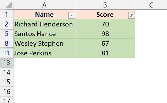
Below I have a data set where I have some rows that are highlighted in green color, and I want to filter these records.

Filter by Cell Color

Here are the steps to do this:

1. Select the data (or any cell in the dataset)
2. Click the Data tab

3. Click on the Filter icon in the Sort & Filter group. This will apply the filter to the first row in your dataset.

You can also use the keyboard shortcut Control + Shift + L to apply the filters.

4. Click on the Filter icon in the column that has the cells with color. In this case, since the entire row has been covered, you can click on the filter icon for any column.

5. Hover the cursor over the ‘Filter by Color’ option. This will further show a sub-menu of the ‘Filter by Cell Color’ options.

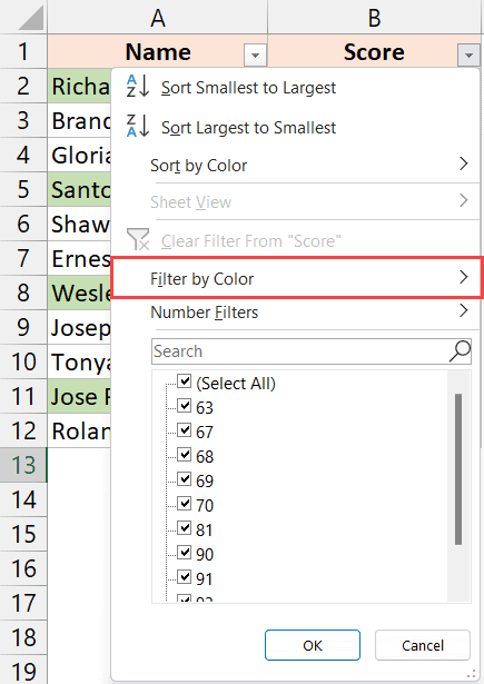
6. Select the color based on which you want to filter this data set. In this example, since we only have one color, only one color is shown in the options. In case you have multiple colors, all would be shown here.

The above steps would instantly filter your data set, and you would only see the records where the specified color is filled in the cell.

One limitation of this method is that you can only filter based on one color. Unlike the text or number filter, the filter-by-color functionality does not allow you to filter based on multiple colors

Also read: How to Count Filtered Rows in Excel?

Filter by Font Color

You can also follow the same steps to filter your data set based on the font color instead of the cell color.

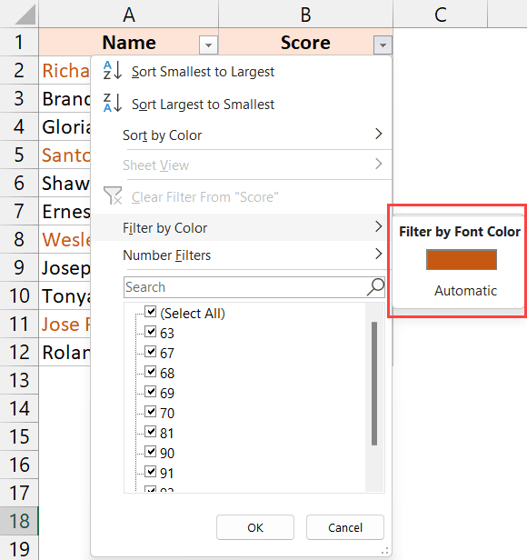
Below I have a data set where I have some records that are in red font color, and I want to filter all these records

Here are the steps to do this:

1. Select the data (or any cell in the dataset)
2. Click the Data tab
3. Click on the Filter icon in the Sort & Filter group.

4. Click on the Filter icon in the column with the cells with color.

5. Hover the cursor over the ‘Filter by Color’ option. This will further show a sub-menu of the ‘Filter by Font color’ options.
6. Select the font color based on which you want to filter this data set. In this example, we only have one font color. In case your dataset has more, all the colors would show up.

The above steps will filter the data, and we’ll keep only those records visible that have the selected font color.

Removing the Filter

If you want to remove the color filter, follow the below steps:

1. Click on the filter icon in the column header where you applied the filter. You can also visually see which column has the filter applied as the icon changes from a simple dropdown icon to a filter icon.
2. Select the ‘Clear Filter from…’ option.

Filter By Color Using Right-click Menu

Another fast way to filter by color is by using the filter option that appears when you right-click on the cell that has the color.

Let me show you how it works.

Filter by Cell Color

Below I have the same data set where I have some colored cells that I want to filter.

Here are the steps to filter my color using the right-click menu:

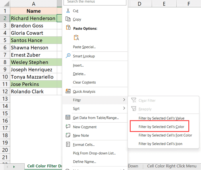
1. Right-click on any of the cells that have the color based on which you want to filter the data

2. Hover the cursor over the Filter option.
3. In the additional options that appear, click on the ‘Filter by Selected Cell’s Color’ option.

That’s it! Your data set would instantly be filtered based on the cell in which you right-clicked.

This method has the same limitation, where you cannot filter based on multiple colors. You can only filter based on one color.

Filter by Font Color

Similarly, you can also quickly filter based on the font color by simply right-clicking on the cell and then choosing the right filter option.

Below I have a data set where I have some cells that are in red font color, and I want to filter these records.

Here are the steps to do this:

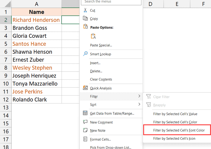
1. Right-click on any of the cells that have the font color based on which you want to filter
2. Hover the cursor over the Filter option.
3. In the additional options that appear, click on the ‘Filter by Selected Cell’s Font Color’ option.

Removing the Filter

Below are the steps to remove the cell color or font color filter:

1. Right-click on any of the cells in the column that has been filtered
2. Hover the cursor over the Filter option
3. Select the ‘Clear Filter from…’ option.

Filter By Color Using VBA

While the above two methods are fast and easy, a big limitation is that you can only filter your data set based on one single color.

But what if you have multiple colors in your data set and you want to filter your data to get records that are highlighted in two or more colors?

Let me show you a very simple VBA code and a smart technique to do this.

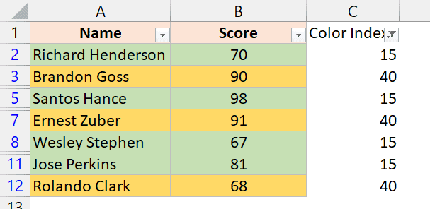
Below, I have a data set where I have cells highlighted in two colors (green and orange), and I want to filter all the records that have green and orange colors.

Since I cannot do this using the regular Filter by Color functionality in Excel, I will add a helper column and then extract the color index value of each cell color in that helper column.

Once I have these values in the helper column, I can easily filter based on multiple colors using multiple color index values.

The first step for this would be to create a custom function in VBA and then use that function in the worksheet to get the color index for each cell.

Below are the steps to create the custom function in Excel:

1. Click the Developer tab and then click on the Visual Basic icon. This will open the VB Editor. You can also use the shortcut ALT + F11 (hold the ALT key and then press the F11 key)

2. Click on the Insert option in the menu
3. Click on the Module option. This will insert a new Module for our workbook

4. Copy and paste the below code to the module code window.

'Code developed by Sumit Bansal from https://trumpexcel.com
Function GetCellColor(cell As Range) As Integer
GetCellColor = cell.Interior.ColorIndex
End Function

'Code developed by Sumit Bansal from https://trumpexcel.com
Function GetCellFontColor(cell As Range) As Integer
GetCellFontColor = cell.Font.ColorIndex
End Function

5. Close the VB Editor

With the above steps, we have created two functions using VBA that can now be used in the worksheet as regular functions.

The GetCellColor function will take the cell reference as the input and give us the numerical value that represents the color index of that cell.

And the GetCellFontColor function takes the cell reference as input and gives us the cell font color index value.

Now let’s see how to use these functions in the worksheet to filter our data by color.

6. In cell C1, enter the text ‘ColorIndex”. We are doing this as we need a header for our helper column. You can write any text you want.

7. Enter the below text in cell C2, and then copy it for all the cells in the column.

=GetCellColor(B2)

The numerical value that you see in the helper column represents the color index value of each cell on the left. So 15 represents the green color in our dataset, 40 represents orange, and -4142 represents no color.

Now that we have all the data, we will see how to filter this data set based on multiple colors.

8. Select the entire data set.
9. Click the Data tab
10. Click on the Filter icon. This will apply filters to the entire first row, including the header of the helper column.

11. Click the filter icon in the helper column.

12. Uncheck the options you don’t want to filter for and keep the numbers for the colors for which you want to filter the data. In our example, we will keep 15 and 40 checked (and uncheck all other options).

13. Click on OK

The above steps would filter our data set based on the selected colors.

Once done, you can hide or remove the helper column if you don’t want it.

Note: In case you want to filter the dataset based on the cell font color instead, use the GetCellFontColor function in step 8.

So these are the methods you can use to filter by color in Excel. If you want to filter just by one cell color or font color, then you can use the right-click technique or apply the filter and then use the options in the filter drop-down (as shown in Method 2 and Method 1, respectively).

And if you need to filter based on multiple colors, you will have to create a User-defined function using VBA and then use that function in the worksheet to fetch the color index, which can then be used to apply the filter.

Other Excel articles you may also like:

• Excel Filter Function – Explained with Examples + Video
• Excel VBA Autofilter: A Complete Guide with Examples
• How to Filter Cells that have Duplicate Text Strings (Words) in it
• How to Filter Cells with Bold Font Formatting in Excel (An Easy Guide)
• How to Sum by Color in Excel (Formula & VBA)
• How to Sort By Color in Excel