
Excel has some really amazing functions, but it doesn’t have a function that can sum cell values based on the cell color.
For example, I have the dataset as shown below, and I want to get the sum of all orange and yellow color cells.

Unfortunately, there is no in-built function to do this.
But never say never!
In this tutorial, I will show you three simple techniques you can use to sum by color in Excel.
Let’s dive in!
SUM Cells by Color Using Filter and SUBTOTAL
Let’s start with the easiest one.
Below I have a dataset where I have the employee names and their sales numbers.
And in this dataset, I want to get the sum of all the cells colored in yellow and orange.
While there is no in-built function in Excel to sum values based on cell color, there is a simple workaround that relies on the fact that you can filter cells based on the cell color.
For this method, enter the below formula in cell B17 (or any cell in the same column below the colored cells dataset).
=SUBTOTAL(9,B2:B15)

In the above SUBTOTAL formula, I have used 9 as the first argument, which tells the function that I want to get the sum of the range that is given as the second argument.
But why not just use the SUM formula instead?
This is because when I have the SUBTOTAL formula and I filter the cells to only show those cells that have a specific color in it, the SUBTOTAL formula will show me the sum of visible cells only (something that the SUM formula can not do).
So once you have the SUBTOTAL formula, follow the below steps to get the SUM based on cell color:
- Select any cell in the dataset
- Click the Data tab

- In the Sort and Filter group, click on the Filter icon. This will apply filter to the dataset and you will be able to see the filter icon in the headers
- In the Sales header cell, click on the Filter icon
- Go to the Filter by Color” option
- Select the color based on which you want to filter the dataset.

As soon as you do this, you will notice that the subtotal result changes and it will now only give you the sum of those cells that are visible (which would only be those cells that have the color by which you filtered the dataset).

Similarly, if you filter by some other color in the data set (say orange instead of yellow), the SUBTOTAL function would accordingly adjust and give you the sum of all cells with orange color
Pro Tip: Keyboard shortcut to apply a filter to a dataset is Control + Shift + L (hold the Control and the Shift key, and then press the L key). If using Mac, use Command + Shift + L
Also read: SUM Based on Partial Text Match in Excel (SUMIF)
SUM Cells by Color Using VBA
I mentioned that there is no in-built formula in Excel to sum based on cell color value. However, you can create your own formula to do this using VBA.
With VBA, you can create a custom function that you can keep in the back end, and then use it like any other regular function in the worksheet.
Below is the VBA code that will create that custom function that allows you to sum by color in Excel.
'Code created by Sumit Bansal from https://trumpexcel.com/
'This VBA code created a function that can be used to sum cells based on color
Function SumByColor(SumRange As Range, SumColor As Range)
Dim SumColorValue As Integer
Dim TotalSum As Long
SumColorValue = SumColor.Interior.ColorIndex
Set rCell = SumRange
For Each rCell In SumRange
If rCell.Interior.ColorIndex = SumColorValue Then
TotalSum = TotalSum + rCell.Value
End If
Next rCell
SumByColor = TotalSum
End FunctionTo use this VBA custom function, you will first have to copy this code and paste it in the back end in the VB editor.
Once done, you’ll be able to use this function in the worksheet.
Below are the steps to add this code to the VB editor.
- Click the Developer tab in the ribbon (if you don’t have the Developer tab visible, click here to learn how to get it)
- Click on the Visual Basic icon. This will open the Visual Basic editor of Excel.

- Click the Insert option in the menu
- Click on Module. This will insert a new module and you will be able to see it in the project explorer (a pane on the left that shows all the objects). If you don’t see the Project Explorer pane, click on View and then click on Project Explorer

- Copy the above VBA code and paste it in the newly inserted Module code window

- Close the VB Editor
Now that you have the code in the back end in excel, you will be able to use the function that we created (SumByColor) in the worksheet.
For this function to work, I will need a cell in the worksheet that contains the same color for which I want to get the sum.
In our example, I have done that to cells D2 and D3, where D2 has the yellow color and D3 has the orange color.
Now I can use the below formula in these cells:
=SumByColor($B$2:$B$15,D2)

The above formula takes two arguments:
- The range of cells that have the color that I want to add
- Reference to any cell that contains the color (so that the formula can pick the color index and use that as a condition to add the values)
Note that the formula is dynamic and would automatically update in case you make any changes to the data set (such as changing any value or applying/removing color from some cells). And in case you notice that the formula is not updating, hit the F9 key and it would update.
Since we have used a VBA code in the workbook, it needs to be saved as a macro-enabled workbook (with .XLSM extension).
Pro Tip: If adding cells based on their background color is something you need to do quite often, I recommend you copy and paste this VBA code for the custom formula in the Personal Macro Workbook. This way, that would be available on all your workbooks on your system.
Also read: Filter By Color in Excel
SUM Cells by Color Using GET.CELL
The final method I want to show you include a hidden Excel formula (that not many people know about).
This method uses the GET.CELL function, which can get us the color index value of colored cells.
And once we have the color index value of each cell, we can then use a simple sum if formula to only get the sum of cells with a specific color in it.
It’s not as elegant as the VBA custom function I covered earlier, but if you don’t want to use VBA, then this could be the way to go for you.
GET.CELL is an old Macro 4 function that has been kept in Excel for compatibility reasons, but you won’t find many details about it (as it’s rarely used).
Below I have a dataset where I have colored cells that I want to sum.
For this technique to work, we first need to create a named range that will use the GET.CELL function to give the color value of a colored cell.
Here are the steps to do this:
- Click the Formulas tab in the Ribbon
- In the Defined Names group, click on the ‘Name Manager’

- In the Name Manager dialog box, click on New

- In the ‘New Name dialog box, enter the Name – SumColor

- In the Refers to field, enter the following formula: =GET.CELL(38,$B2)

- Click OK
- Close the Name Manager dialog box
The above steps have created a named range that we can now use in the workbook.
Note: GET.CELL function takes two arguments, the first one is a number that tells the function what information we need, and the second is the cell reference of that cell itself. In this case, I have 38 as the first argument, which would give us the color index value of the referred cell.
Now the second step is to get the color index values of all the colors in column B.
Below are the steps to do this:
- In cell C1, enter the header – Color Index (or anything that you to call it)

- In cell C2, enter the following formula: =SumColor

- Apply the same formula for all the cell in column C (you can use the fill handle or simply copy paste cell C2)

The above steps would give you a value that would represent the color index of the cell in column B (the cell on the left).
SumColor is the named range we created and it uses the GET.CELL function to get the color index value of the cell on the left. You can use this formula in any column, but it should always start from the second cell in that column. For example, instead of column C, you can have this in column H or J, but from the second cells in these columns.
Now that we have a unique number for each color, we can use this to get the SUM of cells based on their color.
Below are the steps to do this:
- In cell E2 and E3, give the cells the color for which you want to get the sum. In my case, I have yellow color in cell E2 and orange in cell E3

- In cell F2, enter the following formula: =SUMIF(C2:C15,SumColor,B2:B15)
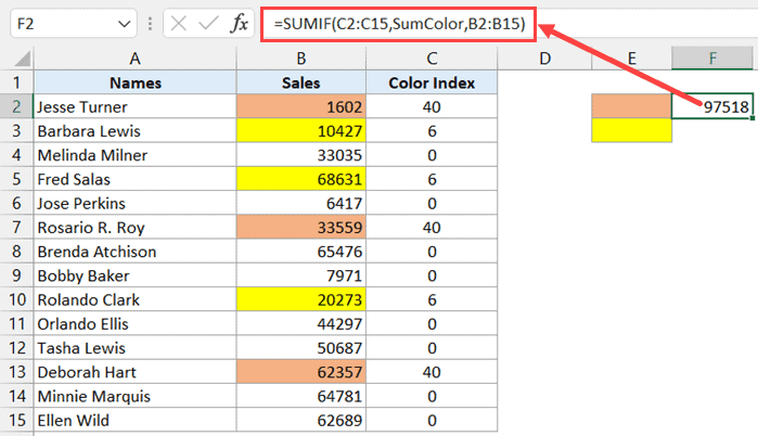
- Copy the cell and paste in cell F3 (this could copy the formula as well and adjust the references).

The above steps would give you the sum of all the cells that have the color in the adjacent selling column F.
We have used a SUMIF formula, where it adds all the values in column B, if the color index of the cell on the left (in column F) is the same as that in column C.
While this is definitely a slightly longer way to sum cells by color (as compared with SUBTOTAL or VBA), this gets the work done, and you only need to do this setup once.
Note that while the formula is dynamic, in case you make any changes (such as changing the color cells in column B or removing the color from it), the change might not be reflected instantly in the SUMIF formula. A simple workaround for it would be to go to the cell that has the formula, click the F2 key to get into the airport, and then hit the enter key. This would force the formula to recalculate and you will get the updated result.
So these are three methods you can use to sum by color in Excel. While SUBTOTAL is quite easy and straightforward, I personally like the VBA method better.
I hope you found this tutorial useful!
Other Excel tutorials you may also like:
- Count Characters in a Cell (or Range of Cells) Using Formulas in Excel
- How to Count Colored Cells in Excel
- How to Sort By Color in Excel (in less than 10 seconds)
- How to Apply Formula to Entire Column in Excel
- How to Sum Only Positive or Negative Numbers in Excel (Easy Formula)
- How to SUM values between two dates (using SUMIFS formula)
- How to Combine Duplicate Rows and Sum the Values in Excel
- How to Sum Across Multiple Sheets in Excel? (3D SUM Formula)


Goodness, I have been screwing around with this for way too long. One short video and you solved my quest. Thank you so much!!
Glad the video helped 🙂
Thank you for this useful summary. BTW, if you use get.cell, it requires saving the file as xlsm.
How do I sum if I have coloured the parallel Column, like Having the numbers in the K column and colour in the J column, and I want the sum of the column K if the J column cell is green or any other colour.
Thank You