Excel 2016 came with a new function – the IFS function.
You can use this function to test multiple conditions at once and then return the result based on it. This is helpful as you don’t have to create those long nested IF formulas that used to get confusing.
Note that the IFS function is available only the Excel 2016 Windows version (and not the Mac version).
When to Use Excel IFS Function
IFS function can test multiple conditions and returns the value as soon as it finds the first condition that is fulfilled.
This makes this function ideal for situations where you need to grade the students based on the marks or find the commission based on the sales values (covered in examples below).
Excel IFS Function – Syntax
=IFS(Condition1, Value1, [Condition2, Value2],…[Condition127, Value127])
- Condition1 – The first condition that is checked.
- Value1 – The value to return if the first condition is TRUE.
- [Condition2….Condition127] – These are optional arguments, and you can use up to 127 conditions in the IFS function.
- [Value2….Value127] – These are optional arguments, and you can use up to 127 values. Each value corresponds to its condition and would be returned if it’s condition is the first one to be TRUE.
Remember that the IFS function would return the value of the first TRUE condition only. So you can have multiple conditions that are TRUE. However, only the value for the first one would be returned.
Additional Notes:
- All the conditions in the IFS function must return either TRUE or FALSE. If it doesn’t, the formula will give an error.
- If all the conditions in the IFS function return FALSE, the result of the formula would be the #N/A error. Since #N/A error is not very helpful in finding out what happened, you can use the last Condition as TRUE, and the value as FALSE or a descriptive text such as “No Match”.
Using Excel IFS Function – Examples
As I mentioned earlier, this function is best suited for situations where you need to check conditions in a sequence and return the value for the first condition that is met.
This makes it ideal for situations where you have to grade students or find commissions for the sales team.
Example 1 – Finding the Grade Based on the Score
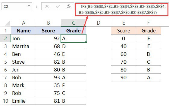
Suppose you have the scores for students in an exam as shown below (column A) and the grading conditions in column C and D.

Below is the formula that will give you the grades for each student:
=IFS(B2<$E$3,$F$2,B2<$E$4,$F$3,B2<$E$5,$F$4,B2<$E$6,$F$5,B2<$E$7,$F$6,B2>$E$7,$F$7)

Looks complicated? Well, to be honest, this is pretty neat as compared to what you would have created had you been using the nested IF formula.
Note that while the cell references of column B are relative, cell references of column E and F have been locked by placing the $ sign (i.e., $E$3). This allows us to copy-paste this formula into all the other cells.
In case you’re using Excel 2013 or prior version (or Excel on Mac), you can get the same result by using the approximate match in the VLOOKUP function. Note that to use VLOOKUP approximate match, the left-most column of the lookup table should be sorted in the ascending order.
Below is the formula that will also give the same result:
=VLOOKUP(B2,$E$2:$F$7,2,1)
Example 2 – Calculating Commission Based on the Sales
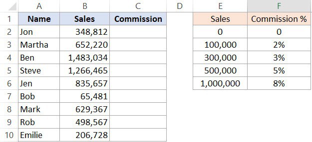
Suppose you’re in charge of the finance department and you have to calculate the commission for each person based on the sales done in the quarter.

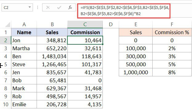
Below is the formula that will give you the commission value for each sales personnel:
=IFS(B2<$E$3,$F$2,B2<$E$4,$F$3,B2<$E$5,$F$4,B2<$E$6,$F$5,B2>$E$6,$F$6)*B2

Related Excel Functions:
- SWITCH Function in Excel
- Excel AND Function.
- Excel OR Function.
- Excel NOT Function.
- Excel IF Function.
- Excel IFERROR Function.
- Excel FALSE Function.
- Excel TRUE Function.
You May Also Like the Following Excel Tutorials:


