
Excel 2010 version of the Pivot Table was jazzed up by the entry of a new super cool feature – Slicers.
A Pivot Table Slicer enables you to filter the data when you select one or more than one options in the Slicer box (as shown below).
In the example above, Slicer is the orange box on the right, and you can easily filter the Pivot Table by simply clicking on the region button in the Slicer.
Let’s get started.
Click here do Download the sample data and follow along.
Inserting a Slicer in Excel Pivot Table
Suppose you have a dataset as shown below:
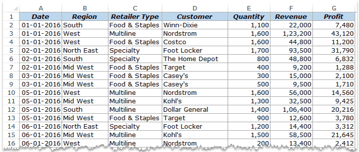
This is a dummy data set (US retail sales) and spans across 1000 rows. Using this data, we have created a Pivot Table that shows the total sales for the four regions.

Read More: How to Create a Pivot Table from Scratch.
Once you have the Pivot Table in place, you can insert Slicers.
One may ask – Why do I need Slicers?
You may need slicers when you don’t want the entire Pivot Table, but only a part of it. For example, if you don’t want to see the sales for all the regions, but only for South, or South and West, then you can insert the slicer and quickly select the desired region(s) for which you want to get the sales data.
Slicers are a more visual way that allows you to filter the Pivot Table data based on the selection.
Here are the steps to insert a Slicer for this Pivot Table:
- Select any cell in the Pivot Table.
- Go to Insert –> Filter –> Slicer.

- In the Insert Slicers dialog box, select the dimension for which you the ability to filter the data. The Slicer Box would list all the available dimensions and you can select one or more than one dimensions at once. For example, if I only select Region, it will insert the Region Slicer box only, and if I select Region and Retailer Type both, then it’ll insert two Slicers.

- Click OK. This will insert the Slicer(s) in the worksheet.
Note that Slicer would automatically identify all the unique items of the selected dimension and list it in the slicer box.
Once you have inserted the slicer, you can filter the data by simply clicking on the item. For example, to get the sales for South region only, click on South. You’ll notice that the selected item gets a different shade of color as compared with the other items in the list.

You can also choose to select multiple items at once. To do that, hold the Control Key and click on the ones that you want to select.

If you want to clear the selection, click on the filter icon (with a red cross) at the top right.

Inserting Multiple Slicers in a Pivot Table
You can also insert multiple slicers by selecting more than one dimension in the Insert Slicers dialog box.
To insert multiple slicers:
- Select any cell in the Pivot Table.
- Go to Insert –> Filter –> Slicer.
- In the Insert Slicers dialog box, select all the dimensions for which you want to get the Slicers.
- Click OK.

This will insert all the selected Slicers in the worksheet.

Note that these slicers are linked to each other. For example, If I select ‘Mid West’ in the Region filter and ‘Multiline’ in the Retailer Type filter, then it will show the sales for all the Multiline retailers in Mid West region only.

Also, if I select Mid West, note that the Specialty option in the second filter gets a lighter shade of blue (as shown below). This indicates that there is no data for Specialty retailer in the Mid West region.

Slicers Vs. Report Filters
What’s the difference between Slicers and Report Filters?
Slicers look super cool and are easy to use. Pivot Table’s strength lies in the fact that you don’t need a lot of skill to use it. All you need to do is drag and drop and click here and there and you’ll have a great report ready within seconds.
While Report Filters does the job just fine, Slicers make it even easier for you to filter a pivot table and/or hand it over to anyone without any knowledge of Excel or Pivot Tables. Since its so intuitive, even that person can himself/herself use these Slicers by clicking on it and filtering the data. Since these are visual filters, it’s easy for anyone to get a hang of it, even when they are using it for the first time.
Here are some key differences between Slicers and Report Filters:
- Slicers don’t occupy a fixed cell in the worksheet. You can move these like any other object or shape. Report Filters are tied to a cell.
- Report filters are linked to a specific Pivot Table. Slicers, on the other hand, can be linked to multiple Pivot Tables (as we will see later in this tutorial).
- Since a report filter occupies a fixed cell, it’s easier to automate it via VBA. On the other hand, a slicer is an object and would need a more complex code.
Formatting the Slicer
A Slicer comes with a lot of flexibility when it comes to formatting.
Here are the things that you can customize in a slicer.
Modifying Slicer Colors
If you don’t like the default colors of a slicer, you can easily modify it.
- Select the slicer.
- Go to Slicer Tools –> Options –> Slicer Styles. Here you’ll find a number of different options. Select the one you like and your slicer would instantly get that formatting.

If you don’t like the default styles, you can create you own. To do this, select the New Slicer Style option and specify your own formatting.
Getting Multiple Columns in the Slicer Box
By default, a Slicer has one column and all the items of the selected dimension are listed in it. In case you have many items, Slicer shows a scroll bar that you can use to go through all the items.

You may want to have all the items visible without the hassle of scrolling. You can do that by creating multiple column Slicer.
To do this:
- Select the Slicer.
- Go to Slicer Tools –> Options –> Buttons.
- Change the Columns value to 2.
This will instantly split the items in the Slicer into two column. However, you may get something looking as awful as shown below:

This looks cluttered and the full names are not displayed. To make it look better, you change the size of the slicer and even the buttons within it.
To do this:
- Select the Slicer.
- Go to Slicer Tools –> Options.
- Change Height and Width of the Buttons and the Slicer. (Note that you can also change the size of the slicer by simply selecting it and using the mouse to adjust the edges. However, to change the button size, you need to make the changes in the Options only).

Changing/Removing the Slicer Header
By default, a Slicer picks the field name from the data. For example, if I create a slicer for Regions, the header would automatically be ‘Region’.
You may want to change the header or completely remove it.
Here are the steps:
- Right-click on the Slicer and select Slicer Settings.

- In the Slicer Settings dialog box, change the header caption to what you want.

- Click OK.
This would change the header in the slicer.
If you don’t want to see the header, uncheck the Display Header option in the dialog box.

Sorting Items in the Slicer
By default, the items in a Slicer are sorted in an ascending order in case of text and Older to Newer in the case of numbers/dates.
You can change the default setting and even use your own custom sort criteria.
Here is how to do this:
- Right-click on the Slicer and select Slicer Settings.
- In the Slicer Settings dialog box, you can change the sorting criteria, or use your own custom sorting criteria.

- Click OK.
Read More: How to create custom lists in Excel (to create your own sorting criteria)
Hiding Items with No Data from the Slicer Box
It may happen that some of the items in the Pivot Table have no data in it. In such cases, you can make the Slicers hide that item.
For example, in the image below, I have two Slicers (one for Region and the other for Retailer type). When I select Mid West, Speciality item in the second filter get’s a light blue shade indicating that there is no data in it.
In such cases, you can choose not display it at all.
Here are the steps to do this:
- Right-click on the Slicer in which you want to hide the data and select Slicer Settings.
- In the Slicer Settings dialog box, with the ‘Item Sorting and Filtering’ options, check the option ‘Hide items with no data’.

- Click OK.
Connecting a Slicer to Multiple Pivot Tables
A slicer can be connected to multiple Pivot Tables. Once connected, you can use a single Slicer to filter all the connected Pivot Tables simultaneously.
Remember, to connect different Pivot Tables to a Slicer, the Pivot Tables need to share the same Pivot Cache. This means that these are either created using the same data, or one of the Pivot Table has been copied and pasted as a separate Pivot Table.
Read More: What is Pivot Table Cache and how to use it?
Below is an example of two different Pivot tables. Note that the Slicer in this case only works for the Pivot Table on the left (and has no effect on the one on the right).

To connect this Slicer to both the Pivot Tables:
- Right-click on the Slicer and select Report Connections. (Alternatively, you can also select the slicer and go to Slicer Tools –> Options –> Slicer –> Report Connections).

- In the Report Connections dialog box, you will see all the Pivot Table names that share the same Pivot Cache. Select the ones you want to connect to the Slicer. In this case, I only have two Pivot Tables and I’ve connected both with the Slicer.

- Click OK.
Now your Slicer is connected to both the Pivot Tables. When you make a selection in the Slicer, the filtering would happen in both the Pivot Tables (as shown below).

Creating Dynamic Pivot Charts Using Slicers
Just as you use a Slicer with a Pivot Table, you can also use it with Pivot Charts.
Something as shown below:
Here is how you can create this dynamic chart:
- Select the data and go to Insert –> Charts –> Pivot Chart.

- In the Create Pivot Chart dialog box, make sure you have the range correct and click OK. This will insert a Pivot Chart in a new sheet.

- Make the fields selections (or drag and drop fields into the area section) to get the Pivot chart you want. In this example, we have the chart that shows sales by region for four quarters. (Read here on how to group dates as quarters).
- Once you have the Pivot Chart ready, go to Insert –> Slicer.
- Select the Slicer dimension you want with the Chart. In this case, I want the retailer types so I check that dimension.

- Format the Chart and the Slicer and you’re done.
Note that you can connect multiple Slicers to the same Pivot Chart and you can also connect multiple charts to the same Slicer (the same way we connected multiple Pivot Tables to the same Slicer).
Click here to download the sample data and try it yourself.
You May Also Like the Following Pivot Table Tutorials:
- How to Group Dates in Excel Pivot Table.
- How to Group Numbers in Pivot Table in Excel.
- How to Refresh Pivot Table in Excel.
- Preparing the Source Data For Pivot Table.
- How to Add and Use an Excel Pivot Table Calculated Field.
- How to Apply Conditional Formatting in a Pivot Table in Excel.
- How to Replace Blank Cells with Zeros in Excel Pivot Tables.


