
Having the data in the right format is a crucial step in creating a robust and error-free Pivot Table. If not done the right way, you can end up having a lot of issues with your pivot table.

What is a good design for the Source data for Pivot Table?
Let’s have a look at an example of good source data for a Pivot Table.
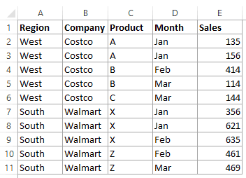
Here’s what makes it a good source data design:
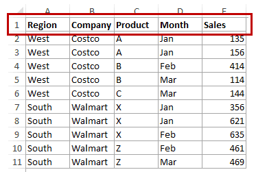
- The first row contains headers that describe the data in the columns.
- Each column represents a unique data category. For example, Column C has product data only and column D and month data only.

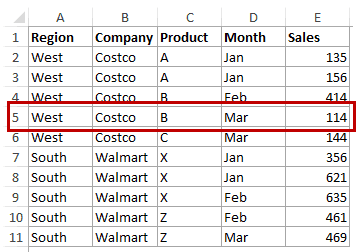
- Each row is a record that would represent one instance of the transaction or sale.
- The Data headers are unique and are not repeated anywhere in the data set. For example, if you have Sales numbers for four quarters in a year, you should NOT name all of these as Sales. Instead, give these column headers unique names such as Sales Q1, Sales Q2, and so on…
- If you don’t have unique titles, you can still go ahead and create a Pivot Table and Excel would automatically make these unique by adding a suffix (such as Sales, Sales2, Sales3). However, that would be an awful way to prepare and use a Pivot Table.

Common Pitfalls to Avoid While Preparing the Source Data
- There shouldn’t be any blank columns in the source data. This one is easy to spot. If you have a blank column in the source data, you wouldn’t be able to create a Pivot Table. It will show an error as shown below.

- There shouldn’t be blanks cells/rows in the source data. While you can successfully create a Pivot Table despite having blank cells or rows, there are many side-effects that can come bite you later in the day.
- For example, let’s say you have a blank cell in the sales column. If you create a Pivot Table using this data and put the sales field in the columns area, it would show you the COUNT and not the SUM. That’s because Excel interprets the entire column as having text data (just because of a single blank cell).

- Apply relevant format to cells in the source data. For example, if you have dates (which are stored as serial numbers in the backend in Excel), apply one of the acceptable date formats. This would help you create the Pivot Table and use Date as one of the criteria to summarize, group, and sort the data.
- If you have a couple of seconds, try this. Format the dates in your Pivot Table as numbers, and then create a Pivot table using this data. Now in the Pivot Table, select the date field and see what happens. It will automatically put it in the values area. That’s because your Pivot Table doesn’t know these are dates. It interprets these as numbers.

- Don’t include any Column Totals, Rows Totals, Averages, etc., as a part of the source data. Once you have the Pivot Table, you can easily get these later.
- Always create an Excel Table and then use it as the source for a Pivot Table. This is more of a good practice and not a pitfall. Your Pivot Table would work just fine with a source data that isn’t an Excel Table as well. The benefit with Excel Table is that it can adjust the expanding data. If you add more rows to the data set, you don’t need to adjust the source data again and again. You can simply refresh the Pivot Table and it would automatically account for the new rows added to the source data.
Also read: Convert Columns to Rows in Excel
Examples of Bad Source Data Designs
Let’s have a look at some bad examples of source data designs.
Bad Source Data Design – Example 1
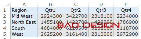
This is a common way to maintain data as it easy to follow and comprehend. There are two problems with this data arrangement:
- You don’t get the complete picture. For example, you can see the sales for Mid West in Quarter 1 is 2924300. But is it a single sale, or a number of sales. If you have each record available in a separate row, you can do a better analysis.
- If you go ahead and create a Pivot Table using this (which you can), you will get different fields for different quarters. Something as shown below:

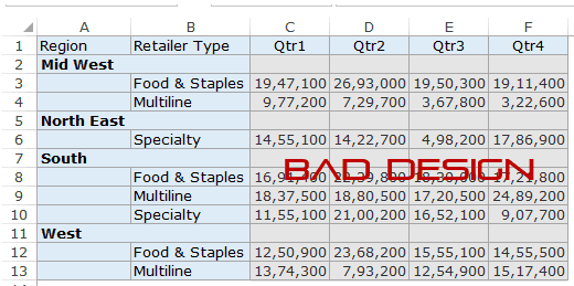
Bad Source Data Design – Example 2
This data representation may be received well by management and the audience of PowerPoint presentations, but it’s not suitable for creating a Pivot Table.
Again, this is the kind of summary that you can easily create using a Pivot Table. So even if you eventually want such a look for your data, maintain the source data in a Pivot ready format and create this view using the Pivot Table.
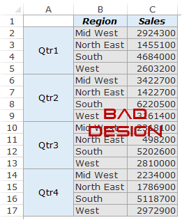
Bad Source Data Design – Example 3
This again is an output that can easily be obtained using a Pivot Table. But it can’t be used to create a Pivot Table.
There are blank cells in the data set and the quarters are spread as column headers.
Also, the region is specified at the top, while it should be a part of every record.
[CASE STUDY] Converting a Badly Formatted Data into Pivot Table Ready Source Data
Sometimes, you may get a dataset that is unsuitable to be used as the source data for Pivot Table. In such a case, you may have no choice but to convert the data into a Pivot friendly data format.
Here is an example of bad data design:
Now you can use Excel Functions or Pivot Query to convert this data into a format that can be used as the source data for Pivot Table.
Let’s see how both of these methods work.
Method 1: Using Excel Formulas
Let’s see how to use Excel Functions to convert this data into a Pivot Table ready format.
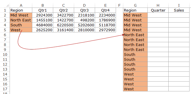
- Create a unique column header for all the categories in the original dataset. In this example, it would be Region, Quarter, and Sales.
- In the cell below the Region header, use the following formula: =INDEX($A$2:$A$5,ROUNDUP(ROWS($A$2:A2)/COUNTA($B$1:$E$1),0))
- Drag the formula down and it will repeat all the regions.
- In the cell below the Quarter header, use the following formula: =INDEX($B$1:$E$1,ROUNDUP(MOD(ROWS($A$2:A2),COUNTA($B$1:$E$1)+0.1),0))
- Drag the formula down and it will repeat all the quarters.
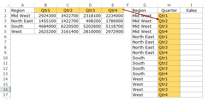
- In the header below Sales, use the following formula: =INDEX($B$2:$E$5,MATCH(G2,$A$2:$A$5,0),MATCH(H2,$B$1:$E$1,0))
- Drag it down to get all the values. This formula uses the Region and the Quarter data as the lookup values and returns the sales value from the original dataset.
Now you can use this resulting data as the source data for Pivot Table.
Click here to download the Example File.
Method 2: Using Power Query
Power Query has a feature that can easily convert this kind of data into Pivot ready data format.
If you’re are using Excel 2016, Power Query features would be available in the Data tab in the Get & Transform group. If you’re using Excel 2013 or prior versions, you can use it as an add-in.
Here is an excellent guide on Installing Power Query by Jon from Excel Campus.
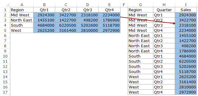
Again, considering you have the data formatted as shown below:
Here are the steps to convert the source data into Pivot Table ready format:
- Convert the data into an Excel Table. Select the dataset and go to Insert –> Tables –> Table.

- In the Insert Table dialog box, make sure the correct range is selected and click OK. This will convert the tabular data into an Excel Table.

- In Excel 2016, go to Data –> Get & Transform –> From Table.
- If you’re using the Power Query Addin in a prior version, go to Power Query –> External Data –> From Table.

- In the Query editor, select the columns that you want to unpivot. In this case, these are the ones for the four quarters. To select all the columns, hold the Shift key and then select the first column and then the last column.

- Within the Query Editor, go to Transform –> Any Column –> Unpivot Columns. This will convert the column’s data into Pivot Table friendly format.

- Power Query gives generic names to the columns. Change these names to the ones you want. In this case, change Attribute to Quarter and Value to Sales.

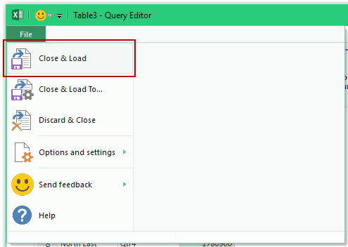
- In the Query Editor, Go to File –> Close and Load. This will close the Power Query Editor dialog box and create a separate worksheet that will have the data with unpivoted columns.
Now that you know how to prepare the source data for Pivot Table you’re ready to Excel in the world of Pivot Tables.
Here are some other Pivot table tutorials that you may find useful:
- How to Refresh Pivot Table in Excel.
- Using Slicers in Excel Pivot Table – A Beginner’s Guide.
- How to Group Dates in Pivot Tables in Excel.
- How to Group Numbers in Pivot Table in Excel.
- Pivot Cache in Excel – What Is It and How to Best Use It.
- How to Filter Data in a Pivot Table in Excel.
- How to Add and Use an Excel Pivot Table Calculated Field.
- How to Apply Conditional Formatting in a Pivot Table in Excel.
- How to Replace Blank Cells with Zeros in Excel Pivot Tables
- Change Pivot Table to Tabular Form


It’s very nice and i need practise Worksheets..
It’s very useful and i want more practise Worksheets…
Many thans for providing us with this valuable information.
Awesome, thanks a lot
Wow – thanks so much for bringing Power Query to my attention – it works perfectly
Nicely developed a layman can create pivot after going through this data. Really thankful trumpexcel.com
how to convert grouped data to pivot friendly data
Great article, Thanks for sharing, keep up the good work!
Hi Sumit,
I have a problem about the table sorting method.
in Method 1: Using Excel Formulas
I’m trying to count the Sales quantity is over 16, the error comes up & shows #REF, Why? Please help on this
And Also, When i use the second formula. if the slaes quantity is like 41,82,123,164,205,246…
there are alway come to the error. and the result will Quarter1 anagin.
Hi Sumit,
Thanks for the cool tip. There is also another method to unpivot data.One can do so by creating pivot table with multiple ranges and double clicking on grand total. Please give a try.
Thanks for commenting Rudra.. That’s a good tip and works great!
HI Sumit,
There is an error in your forumla based solution for this table sorting method.
As you will notice you have used a sequential indexing formula for both the columns. This results in Mid West always getting Qtr1 and North East always getting Qtr2 and so on for all 4 categories. One of the columns needs to be a non-sequential repeating formula.
So I suggest =INDEX($A$2:$A$5,ROUNDUP(ROWS(A$9:A9)/COUNTA($B$1:$E$1),0)) in cell G2 and copy that down all the way. This will repeat Mid West 4 times and then North East 4 times and so on for all 4 categories.
Thanks for pointing it out Abhijeet.. I have updated the tutorial and corrected it. You’re awesome!