
Excel MOD Function (Example + Video)

When to use Excel MOD Function
MOD function can be used when you want to get the remainder when one number is divided by another number.
What it Returns
It returns a numerical value that represents the remainder when one number is divided by another.
Syntax
=MOD(number, divisor)
Input Arguments
- number – A numeric value for which you want to find the remainder.
- divisor – A number with which you want to divide the number argument. If the divisor is 0, then it will return the #DIV/0! error.
Additional Notes
- If the divisor is 0, then it will return the #DIV/0! error.
- The result always has the same sign as that of the divisor.
- You can use decimal numbers in the MOD function. For example, if you use the function =MOD(10.5,2.5), it will return 0.5.
Examples of Using MOD Function in Excel
Here are useful examples of how you can use the MOD function in Excel.
Example 1 – Add Only the Odd or the Even Numbers
Suppose you have a dataset as shown below:

Here is the formula you can use to add only the even numbers:
=SUMPRODUCT($A$2:$A$11*(MOD($A$2:$A$11,2)=0))
Note that here I have hard coded the range ($A$2:$A$11). If your data is likely to change, you can use an Excel Table or created a dynamic named range.
Similarly, if you want to add only the odd numbers, use the below formula:
=SUMPRODUCT($A$2:$A$11*(MOD($A$2:$A$11,2)=1))

This formula works by calculating the remainder using the MOD function.
For example, when calculating the sum of odd numbers, (MOD($A$2:$A$11,2)=1) would return an array of TRUEs and FALSEs. If the number is odd, it would return a TRUE, else a FALSE.
SUMPRODUCT function then only adds those numbers that are returning a TRUE (i.e., odd numbers).
The same concept works when calculating the sum of even numbers.
Example 2 – Specify a Number in Every Nth Cell
Suppose you are making a list of fix expenses every month as shown below:

While the house and car EMIs are monthly, the insurance premium is paid every three months.
You can use the MOD function to quickly fill the cell in every third row with the EMI value.
Here is the formula that will do this:
=IF(MOD((ROW()-1),3)=0,457,””)

This formula simply analyzes the number given by ROW()-1.
ROW function gives us the row number and we have subtracted 1 as our data starts from second row onwards. Now the MOD function checks the remainder when this value is divided by 3.
It will be 0 for every third row. Whenever this is the case, IF function would return 457, else it will return a blank.
Example 3 – Highlight Alternate Rows in Excel
Highlighting alternate rows can increase the readability of your data set (especially when it’s printed).
Something as shown below:

Note that every second row of the dataset is highlighted.
While you can do this manually for a small dataset, if you have a huge one, you can leverage the power of conditional formatting with the MOD function.
Here are the steps that will highlight every second row in the dataset:
- Select the entire data set.
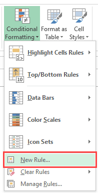
- Go to the Home tab.
- Click on Conditional Formatting and select New Rule.
- In the ‘New Formatting Rule’ dialog box, select ‘Use a formula to determine which cells to format’.
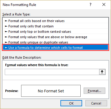
- In the formula field, enter the following formula: =MOD(ROW()-1,2)=0

- Click on the Format button and specify the color in which you want the rows highlighted.
- Click OK.
This will instantly highlight alternate rows in the dataset.
You can read more about this technique and variations of it in this tutorial.
Example 4 – Highlight All the Integer /Decimal Values
You can use the same conditional formatting concept shown above to highlight integer values or decimal values in a data set.
For example, suppose you have a dataset as shown below:

There are numbers that are integers and some of these have decimal values as well.
Here are the steps to highlight all the numbers that have decimal value in it:
- Select the entire data set.
- Go to the Home tab.
- Click on Conditional Formatting and select New Rule.
- In the ‘New Formatting Rule’ dialog box, select ‘Use a formula to determine which cells to format’.
- In the formula field, enter the following formula: =MOD(A1,1)<>0
- Click on the Format button and specify the color in which you want the rows highlighted.
- Click OK.
This will highlight all the numbers that have a decimal part to it.

Note that we in this example, we have used the formula =MOD(A1,1)<>0. In this formula, make sure the cell reference is absolute (i.e., A1) and not relative (i.e., it shouldn’t be $A$1, $A1 or A$1).
Excel MOD Function – Video Tutorial
Related Excel Functions:


I am a little confused about the statement in example 4 on using absolute cell references in the conditional formatting formula. The example given, cell A1, with text saying this is an absolute reference is contradictory to the linked cell reference article. The linked article says a cell reference with no $ signs is a relative reference while a cell reference with $ signs is an absolute reference.
The exact text from above article is: “In this formula, make sure the cell reference is absolute (i.e., A1) and not relative (i.e., it shouldn’t be $A$1, $A1 or A$1).”
In the linked article ‘Absolute, Relative and Mixed Cell References in Excel’ an absolute cell reference is described as: “A dollar symbol, when added in front of the row and column number, makes it absolute…”
Please will you explain the apparent contradiction of if I am missing something.