
Below is the complete written tutorial, in case you prefer reading over watching a video.
Conditional Formatting in Excel can be a great ally in while working with spreadsheets.
A trick as simple as the one to highlight every other row in Excel could immensely increase the readability of your data set.
And it is as EASY as PIE.
Suppose you have a dataset as shown below:
Let’s say you want to highlight every second month (i.e., February, April and so on) in this data set.
This can easily be achieved using conditional formatting.
Highlight Every Other Row in Excel
Here are the steps to highlight every alternate row in Excel:
- Select the data set (B4:D15 in this case).
- Open the Conditional Formatting dialogue box (Home–> Conditional Formatting–> New Rule) [Keyboard Shortcut – Alt + O + D].
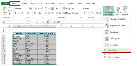
- In the dialogue box, click on “Use a Formula to determine which cells to format” option.


- Click on the Format button to set the formatting.

- Click OK.

That’s it!! You have the alternate rows highlighted.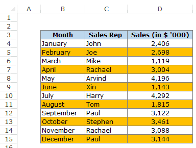
How does it Work?
Now let’s take a step back and understand how this thing works.
The entire magic is in the formula =MOD(ROW(),2)=1. [MOD formula returns the remainder when the ROW number is divided by 2].
This evaluates each cell and checks if it meets the criteria. So it first checks B4. Since the ROW function in B4 would return 4, =MOD(4,2) returns 0, which does not meet our specified criteria.
So it moves on to the other cell in next row.
Here Row number of cell B5 is 5 and =MOD(5,1) returns 1, which meets the condition. Hence, it highlights this entire row (since all the cells in this row have the same row number).
You can change the formula according to your requirements. Here are a few examples:
- Highlight every 2nd row starting from the first row =MOD(ROW(),2)=0
- Highlight every 3rd Row =MOD(ROW(),3)=1
- Highlight every 2nd column =MOD(COLUMN(),2)=0
These banded rows are also called zebra lines and are quite helpful in increasing the readability of the data set.
If you plan to print this, make sure you use a light shade to highlight the rows so that it is readable.
Bonus Tip: Another quick way to highlight alternate rows in Excel is to convert the data range into an Excel Table. As a part of the Excl Table formatting, you can easily highlight alternate rows in Excel (all you need is to use the check the Banded Rows option as shown below):

You May Also Like the Following Excel Tutorials:
- Creating a Heat Map in Excel.
- How to Apply Conditional Formatting in a Pivot Table in Excel.
- Conditional Formatting to Create 100% Stacked Bar Chart in Excel.
- How to Insert Multiple Rows in Excel.
- How to Count Colored Cells in Excel.
- How to Highlight Blank Cells in Excel.
- 7 Quick & Easy Ways to Number Rows in Excel.
- How to Compare Two Columns in Excel.
- Insert a Blank Row after Every Row in Excel (or Every Nth Row)
- Apply Conditional Formatting Based on Another Column in Excel
- Select Every Other Row in Excel


You just saved me days of work in a matter of seconds, THANK YOU SO MUCH
Hi there, thank you your site is very helpful. I work with spreadsheets daily and I like to make my data to be easier on the eyes. Is there a modified formula to =MOD(ROW(),2)=0 so that the 1st row is blank and the shading begins on the 2nd row? Please let me know. THANKS!!!
Sir, 19th March,2020.
I appreciate your efforts to explain deeply each and every lesson.
Generally,what I observed tell you, no one cares to go deeply.
I hope,like me others may have also impressed while reading those articles.
Once again thanking you and hope to receive more and more articles from you in future too.
Kanahaiyalal Newaskar.
If I understand correctly, this is a typo: “Here Row number of cell B5 is 5 and =MOD(5,1) returns 1”; Should this not be “… =MOD(5,2) returns 1”?
Thank you for the site. It is one of the best site I found which caters to a novice to expert Excel user with simple and detailed step by step instructions with examples.
I will definitely recommend it to colleagues and friends.
How do i find % differences between numbers in two columbs?
Sir can you suggest / create any a default function in excel which will highlight row & column for every excel workbook by default without any application.
This was really helpful. Thank you for sharing.
this is what I used to do it years ago…
…but then I discovered Tables
and have never done this again
HOW TO HIGHLIGHT THE CELL IF IT HOLD A SPECIFIC CHARACTER
HOW TO HIGHLIGHT THE CELL OF Nth CAHARACTER
Very Helpful. Thank you for sharing and answering all the questions. This really helped me.
How would you highlight every 10th row, starting from 2?
is there a formula for 4 rows highlighted, 4 rows not highlighted, and so on?
Try this formula:
=ISODD(ROUNDUP(ROW()/4,0))
Awesome thank you! I was just looking for this too 🙂
Hi there, how do I highlight/shade/flag every 5th cell along a single row, and only the cells that contain a ‘1’. I have only found formulas highlighting every nth row down a column, and no examples for along a row. Can you help me?
Try this formula:
=AND((A$1=1),MOD(COLUMN(A$1),5)=0)
How would I do this to highlight every 24th cell -1 (because I don’t want the header accounted for)
Hello Debra.. Do you want to highlight every 23rd row? If yes, you can use this formula =MOD(ROW(),23)=0
Very helpful, thank you so much!
Thanks for commenting. Glad you liked it 🙂
Awesome. Thanks!
Thanks for commenting.. Glad you liked it 🙂
how do you highlight every 15th cell in column H for the SUM mathematical function
Thanks for commenting.. To highlight every 15th cell in column H, select the entire column and use the following formula in conditional formatting
=Mod(row($H1),15)=0
thank you. i forgot to add the range from 712-4430
when i paste the formula it tell me it is false
I guess you are pasting the formula in the worksheet. Instead, you need to paste the formula in the conditional formatting box as shown in the article.
oh ok. thank you. and the range 712-4430
How do I get this to only highlight cells every fourth row that are great than 1 but less than 99999?
Hello Brandy.. Thanks for commenting. To do this select all the cells and use the following formula in conditional formatting
=AND(MOD(ROW(A1),4)=0,A1>0,A1<9999)