
Excel allows having hyperlinks in cells which you can use to directly go to that URL.
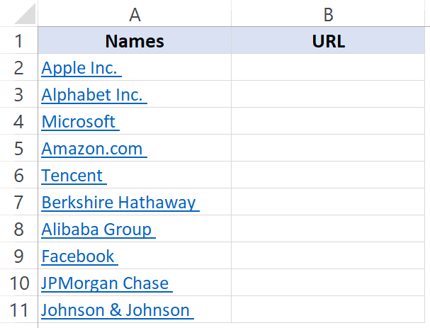
For example, below is a list where I have company names which are hyperlinked to the company website’s URL. When you click on the cell, it will automatically open your default browser (Chrome in my case) and go to that URL.
There are many things you can do with hyperlinks in Excel (such as a link to an external website, link to another sheet/workbook, link to a folder, link to an email, etc.).
In this article, I will cover all you need to know to work with hyperlinks in Excel (including some useful tips and examples).
How to Insert Hyperlinks in Excel
There are many different ways to create hyperlinks in Excel:
- Manually type the URL (or copy paste)
- Using the HYPERLINK function
- Using the Insert Hyperlink dialog box
Let’s learn about each of these methods.
Manually Type the URL
When you manually enter a URL in a cell in Excel, or copy and paste it in the cell, Excel automatically converts it into a hyperlink.
Below are the steps that will change a simple URL into a hyperlink:
- Select a cell in which you want to get the hyperlink
- Press F2 to get into the edit mode (or double click on the cell).
- Type the URL and press enter. For example, if I type the URL – https://trumpexcel.com in a cell and hit enter, it will create a hyperlink to it.

Note that you need to add http or https for those URLs where there is no www in it. In case there is www as the prefix, it would create the hyperlink even if you don’t add the http/https.
Similarly, when you copy a URL from the web (or some other document/file) and paste it in a cell in Excel, it will automatically be hyperlinked.
Insert Using the Dialog Box
If you want the text in the cell to be something else other than the URL and want it to link to a specific URL, you can use the insert hyperlink option in Excel.
Below are the steps to enter the hyperlink in a cell using the Insert Hyperlink dialog box:
- Select the cell in which you want the hyperlink
- Enter the text that you want to be hyperlinked. In this case, I am using the text ‘Sumit’s Blog’
- Click the Insert tab.
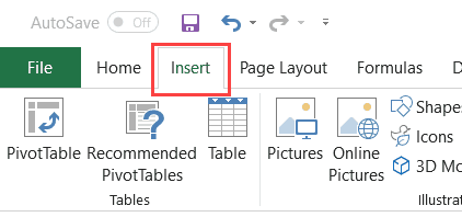
- Click the links button. This will open the Insert Hyperlink dialog box (You can also use the keyboard shortcut – Control + K).

- In the Insert Hyperlink dialog box, enter the URL in the Address field.
- Press the OK button.

This will insert the hyperlink the cell while the text remains the same.

There are many more things you can do with the ‘Insert Hyperlink’ dialog box (such as create a hyperlink to another worksheet in the same workbook, create a link to a document/folder, create a link to an email address, etc.). These are all covered later in this tutorial.
Insert Using the HYPERLINK Function
Another way to insert a link in Excel can be by using the HYPERLINK Function.
Below is the syntax:
HYPERLINK(link_location, [friendly_name])
- link_location: This can be the URL of a web-page, a path to a folder or a file in the hard disk, place in a document (such as a specific cell or named range in an Excel worksheet or workbook).
- [friendly_name]: This is an optional argument. This is the text that you want in the cell that has the hyperlink. In case you omit this argument, it will use the link_location text string as the friendly name.
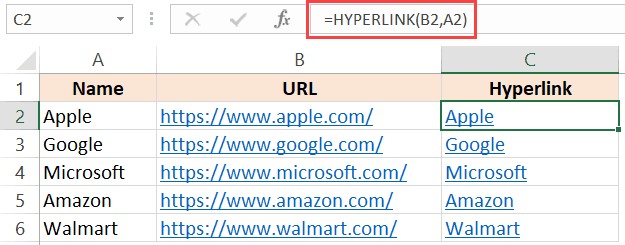
Below is an example where I have the name of companies in one column and their website URL in another column.

Below is the HYPERLINK function to get the result where the text is the company name and it links to the company website.
In the examples so far, we have seen how to create hyperlinks to websites.
But you can also create hyperlinks to worksheets in the same workbook, other workbooks, and files and folders on your hard disk.
Let’s see how it can be done.
Create a Hyperlink to a Worksheet in the Same Workbook
Below are the steps to create a hyperlink to Sheet2 in the same workbook:
- Select the cell in which you want the link
- Enter the text that you want to be hyperlinked. In this example, I have used the text ‘Link to Sheet2’.
- Click the Insert tab.
- Click the links button. This will open the Insert Hyperlink dialog box (You can also use the keyboard shortcut – Control + K).
- In the Insert Hyperlink dialog box, select ‘Place in This Document’ option in the left pane.
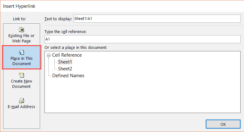
- Enter the cell which you want to hyperlink (I am going with the default A1).

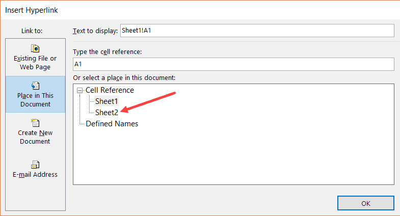
- Select the sheet that you want to hyperlink (Sheet2 in this case)
- Click OK.
Note: You can also use the same method to create a hyperlink to any cell in the same workbook. For example, if you want to link to a far off cell (say K100), you can do that by using this cell reference in step 6 and selecting the existing sheet in step 7.
You can also use the same method to link to a defined name (named cell or named range). If you have any named ranges (named cells) in the workbook, these would be listed in under the ‘Defined Names’ category in the ‘Insert Hyperlink’ dialog box.
Apart from the dialog box, there is also a function in Excel that allows you to create hyperlinks.
So instead of using the dialog box, you can instead use the HYPERLINK formula to create a link to a cell in another worksheet.
The below formula will do this:
=HYPERLINK("#"&"Sheet2!A1","Link to Sheet2")
Below is how this formula works:
- “#” would tell the formula to refer to the same workbook.
- “Sheet2!A1” tells the formula the cell that should be linked to in the same workbook
- “Link to Sheet2” is the text that appears in the cell.
Create a Hyperlink to a File (in the same or different folders)
You can also use the same method to create hyperlinks to other Excel (and non-Excel) files that are in the same folder or are in other folders.
For example, if you want to open a file with the Test.xlsx which is in the same folder as your current file, you can use the below steps:
- Select the cell in which you want the hyperlink
- Click the Insert tab.
- Click the links button. This will open the Insert Hyperlink dialog box (You can also use the keyboard shortcut – Control + K).
- In the Insert Hyperlink dialog box, select ‘Existing File or Webpage’ option in the left pane.
- Select ‘Current folder’ in the Look in options
- Select the file for which you want to create the hyperlink. Note that you can link to any file type (Excel as well as non-Excel files)

- [Optional] Change the Text to Display name if you want to.
- Click OK.
In case you want to link to a file which is not in the same folder, you can Browse the file and then select it. To Browse the file, click on the folder icon in the Insert Hyperlink dialog box (as shown below).

You can also do this using the HYPERLINK function.
The below formula will create a hyperlink that links to a file in the same folder as the current file:
=HYPERLINK("Test.xlsx","Test File")
In case the file is not in the same folder, you can copy the address of the file and use it as the link_location.
Create a Hyperlink to a Folder
This one also follows the same methodology.
Below are the steps to create a hyperlink to a folder:
- Copy the folder address for which you want to create the hyperlink
- Select the cell in which you want the hyperlink
- Click the Insert tab.
- Click the links button. This will open the Insert Hyperlink dialog box (You can also use the keyboard shortcut – Control + K).
- In the Insert Hyperlink dialog box, paste folder address

- Click OK.
You can also use the HYPERLINK function to create a hyperlink that points to a folder.
For example, the below formula will create a hyperlink to a folder named TEST on the desktop and as soon as you click on the cell with this formula, it will open this folder.
=HYPERLINK("C:\Users\sumit\Desktop\Test","Test Folder")
To use this formula, you will have to change the address of the folder to the one you want to link to.
Create Hyperlink to an Email Address
You can also have hyperlinks which open your default email client (such as Outlook) and have the recipients email and the subject line already filled in the send field.
Below are the steps to create an email hyperlink:
- Select the cell in which you want the hyperlink
- Click the Insert tab.
- Click the links button. This will open the Insert Hyperlink dialog box (You can also use the keyboard shortcut – Control + K).
- In the insert dialog box, click on ‘E-mail Address’ in the ‘Link to’ options
- Enter the E-mail address and the Subject line

- [Optional] Enter the text you want to be displayed in the cell.
- Click OK.
Now when you click on the cell which has the hyperlink, it will open your default email client with the email and subject line pre-filled.
You can also do this using the HYPERLINK function.
The below formula will open the default email client and have one email address already pre-filled.
=HYPERLINK("mailto:abc@trumpexcel.com","Send Email")
Note that you need to use mailto: before the email address in the formula. This tells the HYPERLINK function to open the default email client and use the email address that follows.
In case you want to have the subject line as well, you can use the below formula:
=HYPERLINK("mailto:abc@trumpexcel.com,?cc=&bcc=&subject=Excel is Awesome","Generate Email")
In the above formula, I have kept the cc and bcc fields as empty, but you can also these emails if needed.
Here is a detailed guide on how to send emails using the HYPERLINK function.
Remove Hyperlinks
If you only have a few hyperlinks, you can remove these manually, but if you have a lot, you can use a VBA Macro to do this.
Manually Remove Hyperlinks
Below are the steps to remove hyperlinks manually:
- Select the data from which you want to remove hyperlinks.
- Right-click on any of the selected cell.
- Click on the ‘Remove Hyperlink’ option.

The above steps would instantly remove hyperlinks from the selected cells.
In case you want to remove hyperlinks from the entire worksheet, select all the cells and then follow the above steps.
Remove Hyperlinks Using VBA
Below is the VBA code that will remove the hyperlinks from the selected cells:
Sub RemoveAllHyperlinks()
'Code by Sumit Bansal @ trumpexcel.com
Selection.Hyperlinks.Delete
End SubIf you want to remove all the hyperlinks in the worksheet, you can use the below code:
Sub RemoveAllHyperlinks()
'Code by Sumit Bansal @ trumpexcel.com
ActiveSheet.Hyperlinks.Delete
End Sub
Note that this code will not remove the hyperlinks created using the HYPERLINK function.
You need to add this VBA code in the regular module in the VB Editor.
If you need to remove hyperlinks quite often, you can use the above VBA codes, save it in the Personal Macro Workbook, and add it to your Quick Access Toolbar. This will allow you to remove hyperlinks with a single click and it will be available in all the workbooks on your system.
Here is a detailed guide on how to remove hyperlinks in Excel.
Prevent Excel from Creating Hyperlinks Automatically
For some people, it’s a great feature that Excel automatically converts a URL text to a hyperlink when entered in a cell.
And for some people, it’s an irritation.
If you’re in the latter category, let me show you a way to prevent Excel from automatically creating URLs into hyperlinks.
The reason this happens as there is a setting in Excel that automatically converts ‘Internet and network paths’ into hyperlinks.
Here are the steps to disable this setting in Excel:
- Click the File tab.
- Click on Options.

- In the Excel Options dialog box, click on ‘Proofing’ in the left pane.

- Click on the AutoCorrect Options button.

- In the AutoCorrect dialog box, select the ‘AutoFormat As You Type’ tab.

- Uncheck the option – ‘Internet and network paths with hyperlinks’

- Click OK.
- Close the Excel Options dialog box.
If you’ve completed the following steps, Excel would not automatically turn URLs, email address, and network paths into hyperlinks.
Note that this change is applied to the entire Excel application, and would be applied to all the workbooks that you work with.
Extract Hyperlink URLs (using VBA)
There is no function in Excel that can extract the hyperlink address from a cell.
However, this can be done using the power of VBA.
For example, suppose you have a dataset (as shown below) and you want to extract the hyperlink URL in the adjacent cell.
Let me show you two techniques to extract the hyperlinks from the text in Excel.
Extract Hyperlink in the Adjacent Column
If you want to extract all the hyperlink URLs in one go in an adjacent column, you can so that using the below code:
Sub ExtractHyperLinks()
Dim HypLnk As Hyperlink
For Each HypLnk In Selection.Hyperlinks
    HypLnk.Range.Offset(0, 1).Value = HypLnk.Address
Next HypLnk
End SubThe above code goes through all the cells in the selection (using the FOR NEXT loop) and extracts the URLs in the adjacent cell.
In case you want to get the hyperlinks in the entire worksheet, you can use the below code:
Sub ExtractHyperLinks()
On Error Resume Next
Dim HypLnk As Hyperlink
For Each HypLnk In ActiveSheet.Hyperlinks
    HypLnk.Range.Offset(0, 1).Value = HypLnk.Address
Next HypLnk
End SubNote that the above codes wouldn’t work for hyperlinks created using the HYPERLINK function.
Extract Hyperlink Using a Formula (created with VBA)
The above code works well when you want to get the hyperlinks from a dataset in one go.
But if you have a list of hyperlinks that keeps expanding, you can create a User Defined Function/formula in VBA.
This will allow you to quickly use the cell as the input argument and it will return the hyperlink address in that cell.
Below is the code that will create a UDF for getting the hyperlinks:
Function GetHLink(rng As Range) As String
    If rng(1).Hyperlinks.Count <> 1 Then
        GetHLink = ""
    Else
        GetHLink = rng.Hyperlinks(1).Address
    End If
End FunctionNote that this wouldn’t work with Hyperlinks created using the HYPERLINK function.
Also, in case you select a range of cells (instead of a single cell), this formula will return the hyperlink in the first cell only.
Find Hyperlinks with Specific Text
If you’re working with a huge dataset that has a lot of hyperlinks in it, it could be a challenge when you want to find the ones that have a specific text in it.
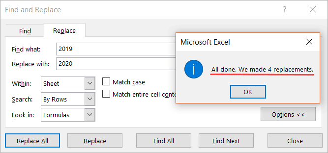
For example, suppose I have a dataset as shown below and I want to find all the cells with hyperlinks that have the text 2019 in it and change it to 2020.

And no.. doing this manually is not an option.
You can do that using a wonderful feature in Excel – Find and Replace.
With this, you can quickly find and select all the cells that have a hyperlink and then change the text 2019 with 2020.
Below are the steps to select all the cells with a hyperlink and the text 2019:
- Select the range in which you want to find the cells with hyperlinks with 2019. In case you want to find in the entire worksheet, select the entire worksheet (click on the small triangle at the top left).
- Click the Home tab.

- In the Editing group, click on Find and Select

- In the drop-down, click on Replace. This will open the Find and Replace dialog box.

- In the Find and Replace dialog box, click on the Options button.This will show more options in the dialog box.

- In the ‘Find What’ options, click on the little downward pointing arrow in the Format button (as shown below).
- Click on the ‘Choose Format From Cell’. This will turn your cursor into a plus icon with a format picker icon.

- Select any cell which has a hyperlink in it. You will notice that the Format gets visible in the box on the left of the Format button. This indicates that the format of the cell you selected has been picked up.

- Enter 2019 in the ‘Find What’ field and 2020 in the ‘Replace with’ field.

- Click on the Replace All button.

In the above data, it will change the text of four cells that have the text 2019 in it and also has a hyperlink.
You can also use this technique to find all the cells with hyperlinks and get a list of it. To do this, instead of clicking on Replace All, click on the Find All button. This will instantly give you a list of all the cell address that has hyperlinks (or hyperlinks with specific text depending on what you’ve searched for).
Note: This technique works as Excel is able to identify the formatting of the cell that you select and use that as a criterion to find cells. So if you’re finding hyperlinks, make sure you select a cell that has the same kind of formatting. If you select a cell that has a background color or any text formatting, it may not find all the correct cells.
Selecting a Cell that has a Hyperlink in Excel
While Hyperlinks are useful, there are a few things about it that irritate me.
For example, if you want to select a cell that has a hyperlink in it, Excel would automatically open your default web browser and try to open this URL.
Another irritating thing about it is that sometimes when you have a cell that has a hyperlink in it, it makes the entire cell clickable. So even if you’re clicking on the hyperlinked text directly, it still opens the browser and the URL of the text.
So let me quickly show you how to get rid of these minor irritants.
Select the Cell (without opening the URL)
This is a simple trick.
When you hover the cursor over a cell that has a hyperlink in it, you’ll notice the hand icon (which indicates if you click on it, Excel will open the URL in a browser)
Click the cell anyway and hold the left button of the mouse.
After a second, you’ll notice that the hand cursor icon changes into the plus icon, and now when you leave it, Excel will not open the URL.
Instead, it would select the cell.
Now, you can make any changes in the cell you want.
Neat trick… right?
Select a Cell by clicking on the blank space in the cell
This is another thing that might drive you nuts.
When there is a cell with the hyperlink in it as well as some blank space, and you click on the blank space, it still opens the hyperlink.
Here is a quick fix.
This happens when these cells have the wrap text enabled.
If you disable wrap text for these cells, you will be able to click on the white space on the right of the hyperlink without opening this link.
Some Practical Example of Using Hyperlink
There are useful things you can do when working with hyperlinks in Excel.
In this section, I am going to cover some examples that you may find useful and can use in your day-to-day work.
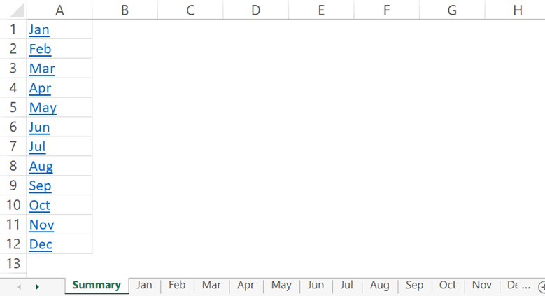
Example 1 – Create an Index of All Sheets in the Workbook
If you have a workbook with a lot of sheets, you can use a VBA code to quickly create a list of the worksheets and hyperlink these to the sheets.
This could be useful when you have 12-month data in 12 different worksheets and want to create one index sheet that links to all these monthly data worksheets.
Below is the code that will do this:
Sub CreateSummary()
'Created by Sumit Bansal of trumpexcel.com
'This code can be used to create summary worksheet with hyperlinks
Dim x As Worksheet
Dim Counter As Integer
Counter = 0
For Each x In Worksheets
Counter = Counter + 1
If Counter = 1 Then GoTo Donothing
    With ActiveCell
        .Value = x.Name
        .Hyperlinks.Add ActiveCell, "", x.Name & "!A1", TextToDisplay:=x.Name, ScreenTip:="Click here to go to the Worksheet"
        With Worksheets(Counter)
            .Range("A1").Value = "Back to " & ActiveSheet.Name
            .Hyperlinks.Add Sheets(x.Name).Range("A1"), "", _
            "'" & ActiveSheet.Name & "'" & "!" & ActiveCell.Address, _
            ScreenTip:="Return to " & ActiveSheet.Name
        End With
    End With
ActiveCell.Offset(1, 0).Select
Donothing:
Next x
End SubYou can place this code in the regular module in the workbook (in VB Editor)
This code also adds a link to the summary sheet in cell A1 of all the worksheets. In case you don’t want that, you can remove that part from the code.
You can read more about this example here.
Note: This code works when you have the sheet (in which you want the summary of all the worksheets with links) at the beginning. In case it’s not at the beginning, this may not give the right results).
Example 2 – Create Dynamic Hyperlinks
In most cases, when you click on a hyperlink in a cell in Excel, it will take you to a URL or to a cell, file or folder. Normally, these are static URLs which means that a hyperlink will take you to a specific predefined URL/location only.
But you can also use a little bit for Excel formula trickery to create dynamic hyperlinks.
By dynamic hyperlinks, I mean links that are dependent on a user selection and change accordingly.
For example, in the below example, I want the hyperlink in cell E2 to point to the company website based on the drop-down list selected by the user (in cell D2).

This can be done using the below formula in cell E2:
=HYPERLINK(VLOOKUP(D2,$A$2:$B$6,2,0), "Click here")
The above formula uses the VLOOKUP function to fetch the URL from the table on the left. The HYPERLINK function then uses this URL to create a hyperlink in the cell with the text – ‘Click here’.
When you change the selection using the drop-down list, the VLOOKUP result will change and would accordingly link to the selected company’s website.
This could be a useful technique when you’re creating a dashboard in Excel. You can make the hyperlinks dynamic depending on the user selection (which could be a drop-down list or a checkbox or a radio button).
Here is a more detailed article of using Dynamic Hyperlinks in Excel.
Example 3 – Quickly Generate Simple Emails Using Hyperlink Function
As I mentioned in this article earlier, you can use the HYPERLINK function to quickly create simple emails (with pre-filled recipient’s emails and the subject line).
Single Recipient Email Id
=HYPERLINK("mailto:abc@trumpexcel.com","Generate Email")
This would open your default email client with the email id abc@trumpexcel.com in the ‘To’ field.
Multiple Recipients Email Id
=HYPERLINK("mailto:abc@trumpexcel.com,def@trumpexcel.com","Generate Email")
For sending the email to multiple recipients, use a comma to separate email ids. This would open the default email client with all the email ids in the ‘To’ field.
Add Recipients in CC and BCC List
=HYPERLINK("mailto:abc@trumpexcel.com,def@trumpexcel.com?cc=123@trumpexcel.com&bcc=456@trumpexcel.com","Generate Email")
To add recipients to CC and BCC list, use question mark ‘?’ when ‘mailto’ argument ends, and join CC and BCC with ‘&’. When you click on the link in excel, it would have the first 2 ids in ‘To’ field, 123@trumpexcel.com in ‘CC’ field and 456@trumpexcel.com in the ‘BCC’ field.
Add Subject Line
=HYPERLINK("mailto:abc@trumpexcel.com,def@trumpexcel.com?cc=123@trumpexcel.com&bcc=456@trumpexcel.com&subject=Excel is Awesome","Generate Email")
You can add a subject line by using the &Subject code. In this case, this would add ‘Excel is Awesome’ in the ‘Subject’ field.
Add Single Line Message in Body
=HYPERLINK("mailto:abc@trumpexcel.com,def@trumpexcel.com?cc=123@trumpexcel.com&bcc=456@trumpexcel.com&subject=Excel is Awesome&body=I love Excel","Email Trump Excel")
This would add a single line ‘I love Excel’ to the email message body.
Add Multiple Lines Message in Body
=HYPERLINK("mailto:abc@trumpexcel.com,def@trumpexcel.com?cc=123@trumpexcel.com&bcc=456@trumpexcel.com&subject=Excel is Awesome&body=I love Excel.%0AExcel is Awesome","Generate Email")
To add multiple lines in the body you need to separate each line with %0A. If you wish to introduce two line breaks, add %0A twice, and so on.
Here is a detailed article on how to send emails from Excel.
Hope you found this article useful.
Let me know your thoughts in the comments section.
You May Also Like the Following Excel Tutorials:


Dear Sumit Bansal, your “Example 1 – Create an Index of All Sheets in the Workbook” has an error and works not correctly.
#1 if the sheets has “(” or space ” ” in the name, the links in the Summary sheet are wrong. You get an error message after clicking them. Try simple Excel Workbook with Sheets named “S”, “S(2)” and “S 3” for example.
#2 the Summary sheet in my opinion should be generated automatically AND more important active cell set to A1. You do either one nor second.
Whatt follows is a summary elswhere in the active sheet (after the active cell of course).
The code example is only partially usefull – I would not publish it (I was programmer since 1977, now retired). Best regards
Sir, 11th July,2020.
Very neatly and clearly you have shown the article ” Hyperlink”.
I must salute your efforts.
Moreover, I eagerly await such Tips and Tricks in near future too.
Once again thanking you.
Kanhaiyalal Newaskar.
How to return a value when click on a hyper link. For example value in Sheet1 A1 is “Test” and there is an hyperlink to sheet2 A1 , so after when click, the value “Test1” should reflect in Sheet2 A1..
I would like to be able to hover over a hyperlink and display specific text. How can I do that?
Hi. Thanks for the excellent tutorial on hyperlinks. I am trying to record a macro in excel that inserts a dynamic hyperlink into an image which is then added to an email. The only part that I am stuck on is when using the “Insert Hyperlink” dialogue box, I can’t paste the URL into the address tab. All of the options are greyed out. Interestingly, when I do the same action within Outlook, I CAN paste the URL into the dialogue box if I try to insert within Outlook. Any tips on what is causing the dialogue box in excel to grey out the paste functions? Any help much appreciated – Thanks.
The marcos here are lifesavers. Thank you!
Is it possible to link a portion of the sheet to email directly to an email by simply clicking the hyperlink? i.e if i have several data sets that need to go to different people in a single sheet. I cannot just send the entire sheet for privacy reasons.
how to link a folder contains multiple jpg photos with serial number 1 to so on such as 1.JPG,2.JPG,…