24 Useful Excel Macro Examples for VBA Beginners

Using Excel Macros can speed up work and save you a lot of time.

One way of getting the VBA code is to record the macro and take the code it generates. However, that code by macro recorder is often full of code that is not really needed. Also macro recorder has some limitations.

So it pays to have a collection of useful VBA macro codes that you can have in your back pocket and use it when needed.

While writing an Excel VBA macro code may take some time initially, once it’s done, you can keep it available as a reference and use it whenever you need it next.

In this massive article, I am going to list some useful Excel macro examples that I need often and keep stashed away in my private vault.

I will keep updating this tutorial with more macro examples. If you think something should be on the list, just leave a comment.

You can bookmark this page for future reference.

Now before I get into the Macro Example and give you the VBA code, let me first show you how to use these example codes.

Using the Code from Excel Macro Examples

Here are the steps you need to follow to use the code from any of the examples:

• Open the Workbook in which you want to use the macro.
• Hold the ALT key and press F11. This opens the VB Editor.
• Right-click on any of the objects in the project explorer.
• Go to Insert –> Module.
• Copy and Paste the code in the Module Code Window.

In case the example says that you need to paste the code in the worksheet code window, double click on the worksheet object and copy paste the code in the code window.

Once you have inserted the code in a workbook, you need to save it with a .XLSM or .XLS extension.

How to Run the Macro

Once you have copied the code in the VB Editor, here are the steps to run the macro:

• Go to the Developer tab.
• Click on Macros.

• In the Macro dialog box, select the macro you want to run.
• Click on Run button.

In case you can’t find the developer tab in the ribbon, read this tutorial to learn how to get it.

Related Tutorial: Different ways to run a macro in Excel.

In case the code is pasted in the worksheet code window, you don’t need to worry about running the code. It will automatically run when the specified action occurs.

Now, let’s get into the useful macro examples that can help you automate work and save time.

Note: You will find many instances of an apostrophe (‘) followed by a line or two. These are comments that are ignored while running the code and are placed as notes for self/reader.

In case you find any error in the article or the code, please be awesome and let me know.

Excel Macro Examples

Below macro examples are covered in this article:

Unhide All Worksheets at One Go

If you are working in a workbook that has multiple hidden sheets, you need to unhide these sheets one by one. This could take some time in case there are many hidden sheets.

Here is the code that will unhide all the worksheets in the workbook.

'This code will unhide all sheets in the workbook
Sub UnhideAllWoksheets()
Dim ws As Worksheet
For Each ws In ActiveWorkbook.Worksheets
ws.Visible = xlSheetVisible
Next ws
End Sub

The above code uses a VBA loop (For Each) to go through each worksheets in the workbook. It then changes the visible property of the worksheet to visible.

Here is a detailed tutorial on how to use various methods to unhide sheets in Excel.

Hide All Worksheets Except the Active Sheet

If you’re working on a report or dashboard and you want to hide all the worksheet except the one that has the report/dashboard, you can use this macro code.

'This macro will hide all the worksheet except the active sheet
Sub HideAllExceptActiveSheet()
Dim ws As Worksheet
For Each ws In ThisWorkbook.Worksheets
If ws.Name <> ActiveSheet.Name Then ws.Visible = xlSheetHidden
Next ws
End Sub

Sort Worksheets Alphabetically Using VBA

If you have a workbook with many worksheets and you want to sort these alphabetically, this macro code can come in really handy. This could be the case if you have sheet names as years or employee names or product names.

'This code will sort the worksheets alphabetically
Sub SortSheetsTabName()
Application.ScreenUpdating = False
Dim ShCount As Integer, i As Integer, j As Integer
ShCount = Sheets.Count
For i = 1 To ShCount - 1
For j = i + 1 To ShCount
If Sheets(j).Name < Sheets(i).Name Then
Sheets(j).Move before:=Sheets(i)
End If
Next j
Next i
Application.ScreenUpdating = True
End Sub

Protect All Worksheets At One Go

If you have a lot of worksheets in a workbook and you want to protect all the sheets, you can use this macro code.

It allows you to specify the password within the code. You will need this password to unprotect the worksheet.

'This code will protect all the sheets at one go
Sub ProtectAllSheets()
Dim ws As Worksheet
Dim password As String
password = "Test123" 'replace Test123 with the password you want
For Each ws In Worksheets
   ws.Protect password:=password
Next ws
End Sub

Unprotect All Worksheets At One Go

If you have some or all of the worksheets protected, you can just use a slight modification of the code used to protect sheets to unprotect it.

'This code will protect all the sheets at one go
Sub ProtectAllSheets()
Dim ws As Worksheet
Dim password As String
password = "Test123" 'replace Test123 with the password you want
For Each ws In Worksheets
ws.Unprotect password:=password
Next ws
End Sub

Note that the password needs to the same that has been used to lock the worksheets. If it’s not, you will see an error.

Unhide All Rows and Columns

This macro code will unhide all the hidden rows and columns.

This could be really helpful if you get a file from someone else and want to be sure there are no hidden rows/columns.

'This code will unhide all the rows and columns in the Worksheet
Sub UnhideRowsColumns()
Columns.EntireColumn.Hidden = False
Rows.EntireRow.Hidden = False
End Sub

Unmerge All Merged Cells

It’s a common practice to merge cells to make it one. While it does the work, when cells are merged you will not be able to sort the data.

In case you are working with a worksheet with merged cells, use the code below to unmerge all the merged cells at one go.

'This code will unmerge all the merged cells
Sub UnmergeAllCells()
ActiveSheet.Cells.UnMerge
End Sub

Note that instead of Merge and Center, I recommend using the Centre Across Selection option.

Save Workbook With TimeStamp in Its Name

A lot of time, you may need to create versions of your work. These are quite helpful in long projects where you work with a file over time.

A good practice is to save the file with timestamps.

Using timestamps will allow you to go back to a certain file to see what changes were made or what data was used.

Here is the code that will automatically save the workbook in the specified folder and add a timestamp whenever it’s saved.

'This code will Save the File With a Timestamp in its name
Sub SaveWorkbookWithTimeStamp()
Dim timestamp As String
timestamp = Format(Date, "dd-mm-yyyy") & "_" & Format(Time, "hh-ss")
ThisWorkbook.SaveAs "C:UsersUsernameDesktopWorkbookName" & timestamp
End Sub

You need to specify the folder location and the file name.

In the above code, “C:UsersUsernameDesktop is the folder location I have used. You need to specify the folder location where you want to save the file. Also, I have used a generic name “WorkbookName” as the filename prefix. You can specify something related to your project or company.

Save Each Worksheet as a Separate PDF

If you work with data for different years or divisions or products, you may have the need to save different worksheets as PDF files.

While it could be a time-consuming process if done manually, VBA can really speed it up.

Here is a VBA code that will save each worksheet as a separate PDF.

'This code will save each worsheet as a separate PDF
Sub SaveWorkshetAsPDF()
Dim ws As Worksheet
For Each ws In Worksheets
ws.ExportAsFixedFormat xlTypePDF, "C:UsersSumitDesktopTest" & ws.Name & ".pdf"
Next ws
End Sub

In the above code, I have specified the address of the folder location in which I want to save the PDFs. Also, each PDF will get the same name as that of the worksheet. You will have to modify this folder location (unless your name is also Sumit and you’re saving it in a test folder on the desktop).

Note that this code works for worksheets only (and not chart sheets).

Save Each Worksheet as a Separate PDF

Here is the code that will save your entire workbook as a PDF in the specified folder.

'This code will save the entire workbook as PDF
Sub SaveWorkshetAsPDF()
ThisWorkbook.ExportAsFixedFormat xlTypePDF, "C:UsersSumitDesktopTest" & ThisWorkbook.Name & ".pdf"
End Sub

You will have to change the folder location to use this code.

Convert All Formulas into Values

Use this code when you have a worksheet that contains a lot of formulas and you want to convert these formulas to values.

'This code will convert all formulas into values
Sub ConvertToValues()
With ActiveSheet.UsedRange
.Value = .Value
End With
End Sub

This code automatically identifies cells are used and convert it into values.

Protect/Lock Cells with Formulas

You may want to lock cells with formulas when you have a lot of calculations and you don’t want to accidentally delete it or change it.

Here is the code that will lock all the cells that have formulas, while all the other cells are not locked.

'This macro code will lock all the cells with formulas
Sub LockCellsWithFormulas()
With ActiveSheet
   .Unprotect
   .Cells.Locked = False
   .Cells.SpecialCells(xlCellTypeFormulas).Locked = True
   .Protect AllowDeletingRows:=True
End With
End Sub

Related Tutorial: How to Lock Cells in Excel.

Protect All Worksheets in the Workbook

Use the below code to protect all the worksheets in a workbook at one go.

'This code will protect all sheets in the workbook
Sub ProtectAllSheets()
Dim ws As Worksheet
For Each ws In Worksheets
ws.Protect
Next ws
End Sub

This code will go through all the worksheets one by one and protect it.

In case you want to unprotect all the worksheets, use ws.Unprotect instead of ws.Protect in the code.

Insert A Row After Every Other Row in the Selection

Use this code when you want to insert a blank row after every row in the selected range.

'This code will insert a row after every row in the selection
Sub InsertAlternateRows()
Dim rng As Range
Dim CountRow As Integer
Dim i As Integer
Set rng = Selection
CountRow = rng.EntireRow.Count
For i = 1 To CountRow
ActiveCell.EntireRow.Insert
ActiveCell.Offset(2, 0).Select
Next i
End Sub

Similarly, you can modify this code to insert a blank column after every column in the selected range.

Automatically Insert Date & Timestamp in the Adjacent Cell

A timestamp is something you use when you want to track activities.

For example, you may want to track activities such as when was a particular expense incurred, what time did the sale invoice was created, when was the data entry done in a cell, when was the report last updated, etc.

Use this code to insert a date and time stamp in the adjacent cell when an entry is made or the existing contents are edited.

'This code will insert a timestamp in the adjacent cell
Private Sub Worksheet_Change(ByVal Target As Range)
On Error GoTo Handler
If Target.Column = 1 And Target.Value <> "" Then
Application.EnableEvents = False
Target.Offset(0, 1) = Format(Now(), "dd-mm-yyyy hh:mm:ss")
Application.EnableEvents = True
End If
Handler:
End Sub

Note that you need to insert this code in the worksheet code window (and not the in module code window as we have done in other Excel macro examples so far). To do this, in the VB Editor, double click on the sheet name on which you want this functionality. Then copy and paste this code in that sheet’s code window.

Also, this code is made to work when the data entry is done in Column A (note that the code has the line Target.Column = 1). You can change this accordingly.

Highlight Alternate Rows in the Selection

Highlighting alternate rows can increase the readability of your data tremendously. This can be useful when you need to take a print out and go through the data.

Here is a code that will instantly highlight alternate rows in the selection.

'This code would highlight alternate rows in the selection
Sub HighlightAlternateRows()
Dim Myrange As Range
Dim Myrow As Range
Set Myrange = Selection
For Each Myrow In Myrange.Rows
   If Myrow.Row Mod 2 = 1 Then
      Myrow.Interior.Color = vbCyan
   End If
Next Myrow
End Sub

Note that I have specified the color as vbCyan in the code. You can specify other colors as well (such as vbRed, vbGreen, vbBlue).

Highlight Cells with Misspelled Words

Excel doesn’t have a spell check as it has in Word or PowerPoint. While you can run the spell check by hitting the F7 key, there is no visual cue when there is a spelling mistake.

Use this code to instantly highlight all the cells that have a spelling mistake in it.

'This code will highlight the cells that have misspelled words
Sub HighlightMisspelledCells()
Dim cl As Range
For Each cl In ActiveSheet.UsedRange
If Not Application.CheckSpelling(word:=cl.Text) Then
cl.Interior.Color = vbRed
End If
Next cl
End Sub

Note that the cells that are highlighted are those that have text that Excel considers as a spelling error. In many cases, it would also highlight names or brand terms that it doesn’t understand.

Refresh All Pivot Tables in the Workbook

If you have more than one Pivot Table in the workbook, you can use this code to refresh all these Pivot tables at once.

'This code will refresh all the Pivot Table in the Workbook
Sub RefreshAllPivotTables()
Dim PT As PivotTable
For Each PT In ActiveSheet.PivotTables
PT.RefreshTable
Next PT
End Sub

You can read more about refreshing Pivot Tables here.

Change the Letter Case of Selected Cells to Upper Case

While Excel has the formulas to change the letter case of the text, it makes you do that in another set of cells.

Use this code to instantly change the letter case of the text in the selected text.

'This code will change the Selection to Upper Case
Sub ChangeCase()
Dim Rng As Range
For Each Rng In Selection.Cells
If Rng.HasFormula = False Then
Rng.Value = UCase(Rng.Value)
End If
Next Rng
End Sub

Note that in this case, I have used UCase to make the text case Upper. You can use LCase for lower case.

Highlight All Cells With Comments

Use the below code to highlight all the cells that have comments in it.

'This code will highlight cells that have comments`
Sub HighlightCellsWithComments()
ActiveSheet.Cells.SpecialCells(xlCellTypeComments).Interior.Color = vbBlue
End Sub

In this case, I have used vbBlue to give a blue color to the cells. You can change this to other colors if you want.

Highlight Blank Cells With VBA

While you can highlight blank cell with conditional formatting or using the Go to Special dialog box, if you have to do it quite often, it’s better to use a macro.

Once created, you can have this macro in the Quick Access Toolbar or save it in your personal macro workbook.

Here is the VBA macro code:

'This code will highlight all the blank cells in the dataset
Sub HighlightBlankCells()
Dim Dataset as Range
Set Dataset = Selection
Dataset.SpecialCells(xlCellTypeBlanks).Interior.Color = vbRed
End Sub

In this code, I have specified the blank cells to be highlighted in the red color. You can choose other colors such as blue, yellow, cyan, etc.

How to Sort Data by Single Column

You can use the below code to sort data by the specified column.

Sub SortDataHeader()
Range("DataRange").Sort Key1:=Range("A1"), Order1:=xlAscending, Header:=xlYes
End Sub

Note that the I have created a named range with the name ‘DataRange’ and have used it instead of the cell references.

Also there are three key parameters that are used here:

• Key1 – This is the on which you want to sort the data set. In the above example code, the data will be sorted based on the values in column A.
• Order- Here you need to specify whether you want to sort the data in ascending or descending order.
• Header – Here you need to specify whether your data has headers or not.

Read more on how to sort data in Excel using VBA.

How to Sort Data by Multiple Columns

Suppose you have a dataset as shown below:

Below is the code that will sort the data based on multiple columns:

Sub SortMultipleColumns()
With ActiveSheet.Sort
 .SortFields.Add Key:=Range("A1"), Order:=xlAscending
 .SortFields.Add Key:=Range("B1"), Order:=xlAscending
 .SetRange Range("A1:C13")
 .Header = xlYes
 .Apply
End With
End Sub

Note that here I have specified to first sort based on column A and then based on column B.

The output would be something as shown below:

How to Get Only the Numeric Part from a String in Excel

If you want to extract only the numeric part or only the text part from a string, you can create a custom function in VBA.

You can then use this VBA function in the worksheet (just like regular Excel functions) and it will extract only the numeric or text part from the string.

Something as shown below:

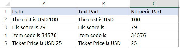
Below is the VBA code that will create a function to extract numeric part from a string:

'This VBA code will create a function to get the numeric part from a string
Function GetNumeric(CellRef As String)
Dim StringLength As Integer
StringLength = Len(CellRef)
For i = 1 To StringLength
If IsNumeric(Mid(CellRef, i, 1)) Then Result = Result & Mid(CellRef, i, 1)
Next i
GetNumeric = Result
End Function

You need place in code in a module, and then you can use the function =GetNumeric in the worksheet.

This function will take only one argument, which is the cell reference of the cell from which you want to get the numeric part.

Similarly, below is the function that will get you only the text part from a string in Excel:

'This VBA code will create a function to get the text part from a string
Function GetText(CellRef As String)
Dim StringLength As Integer
StringLength = Len(CellRef)
For i = 1 To StringLength
If Not (IsNumeric(Mid(CellRef, i, 1))) Then Result = Result & Mid(CellRef, i, 1)
Next i
GetText = Result
End Function

So these are some of the useful Excel macro codes that you can use in your day-to-day work to automate tasks and be a lot more productive.

Other Excel tutorials you may like:

• How to Delete Macros in Excel
• How to Enable Macros in Excel?
• How to Describe Excel Skills in a Resume?