
Text to Columns is an amazing feature in Excel that deserves a lot more credit than it usually gets.
As it’s name suggests, it is used to split the text into multiple columns. For example, if you have a first name and last name in the same cell, you can use this to quickly split these into two different cells.
This can be really helpful when you get your data from databases or you import it from other file formats such as Text or CSV.
In this tutorial, you’ll learn about many useful things that can be done using Text to Columns in Excel.
Where to Find Text to Columns in Excel
To access Text to Columns, select the dataset and go to Data → Data Tools → Text to Columns.

This would open the Convert Text to Columns Wizard.
This wizard has three steps and takes some user inputs before splitting the text into columns (you will see how these different options can be used in examples below).
To access Text to Columns, you can also use the keyboard shortcut – ALT + A + E.
Now let’s dive in and see some amazing stuff you can do with Text to Columns in Excel.
Example 1 – Split Names into the First Name and Last Name
Suppose you have a dataset as shown below:

To quickly split the first name and the last name and get these in separate cells, follow the below steps:
- Select the data set.
- Go to Data → Data Tools → Text to Columns. This will open the Convert Text to Columns Wizard.
- In Step 1, make sure Delimited is selected (which is also the default selection). Click on Next.

- In Step 2, select ‘Space’ as the delimiter. If you suspect that there could be double/triple consecutive spaces between the names, also select ‘Treat consecutive delimiters as one’ option. Click on Next.

- In Step 3, select the destination cell. If you don’t select a destination cell, it would overwrite your existing data set with the first name in the first column and last name in the adjacent column. If you want to keep the original data intact, either create a copy or choose a different destination cell.

- Click on Finish.
This would instantly give you the results with the first name in one column and last name in another column.

Note:
- This technique works well when you the name constitutes of the first name and the last name only. In case there are initials or middle names, then this might not work. Click here for a detailed guide on how to tackle cases with different combinations of names.
- The result you get from using the Text to Columns feature is static. This means that if there are any changes in the original data, you’ll have to repeat the process to get updated results.
Also read: How to Sort by the Last Name in Excel
Example 2 – Split Email Ids into Username and Domain Name
Text to Columns allows you to choose your own delimiter to split text.
This can be used to split emails addresses into usernames and domain names as these are separated by the @ sign.
Suppose you have a dataset as shown below:

These are some fictional email ids of some cool superheroes (except myself, I am just a regular wasting-time-on-Netflix kinda guy).
Here are the steps to split these usernames and domain names using the Text to Columns feature.
- Select the data set.
- Go to Data → Data Tools → Text to Columns. This will open the Convert Text to Columns Wizard.
- In Step 1, make sure Delimited is selected (which is also the default selection). Click on Next.

- In Step 2, select Other and enter @ in the box to the right of it. Make sure to deselect any other option (if checked). Click on Next.

- Change the destination cell to the one where you want the result.

- Click on Finish.
This would split the email address and give you the first name and the last name in separate cells.

Also read: How to Combine 2 Cells in Excel
Example 3 – Get the Root Domain from URL
If you work with web URLs, you may sometimes need to know the total number of unique root domains.
For example, in case of http://www.google.com/example1 and http://google.com/example2, the root domain is the same, which is www.google.com
Suppose you have a dataset as shown below:

Here are the steps to get the root domain from these URLs:
- Select the data set.
- Go to Data → Data Tools → Text to Columns. This will open the Convert Text to Columns Wizard.
- In Step 1, make sure Delimited is selected (which is also the default selection). Click on Next.

- In Step 2, select Other and enter / (forward slash) in the box to the right of it. Make sure to deselect any other option (if checked). Click on Next.

- Change the destination cell to the one where you want the result.
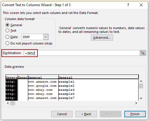
- Click on Finish.
This would split the URL and give you the root domain (in the third column as there were two forward slashes before it).

Now if you want to find the number of unique domains, just remove the duplicates.
Note: This works well when you have all the URLs that have http:// in the beginning. If it doesn’t, then you will get the root domain in the first column itself. A good practice is to make these URLs consistent before using Text to Columns.
Also read: Split Text into Multiple Rows in Excel
Example 4 – Convert Invalid Date Formats Into Valid Date Formats
If you get your data from databases such as SAP/Oracle/Capital IQ, or you import it from a text file, there is a possibility that the date format is incorrect (i.e., a format that Excel does not consider as date).
There are only a couple of formats that Excel can understand, and any other format needs to be converted into a valid format to be used in Excel.
Suppose you have dates in the below format (which are not in the valid Excel date format).

Here are the steps to convert these into valid date formats:
- Select the data set.
- Go to Data → Data Tools → Text to Columns. This will open the Convert Text to Columns Wizard.
- In Step 1, make sure Delimited is selected (which is also the default selection). Click on Next.

- In Step 2, make sure NO delimiter option is selected. Click on Next.
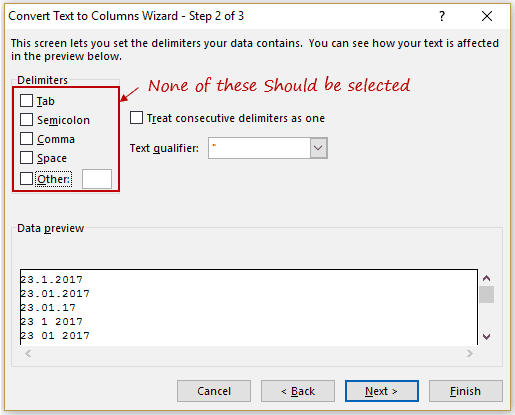
- In the Column data format, select Date, and select the format you want (DMY would mean date month and year). Also, change the destination cell to the one where you want the result.

- Click on Finish.
This would instantly convert these invalid date formats into valid date formats that you can use in Excel.
Example 5 – Convert Text to Numbers
Sometimes when you import data from databases or other file formats, the numbers are converted into text format.
There are several ways this can happen:
- Having an apostrophe before the number. This leads to the number being treated as text.
- Getting numbers as a result of text functions such as LEFT, RIGHT, or MID.
The problem with this is that these numbers (which are in text format) are ignored by Excel functions such as SUM and AVERAGE.
Suppose you have a dataset as shown below where the numbers are in the text format (note that these are aligned to the left).

Here are the steps to use Text to Columns to convert text to numbers
- Select the data set.
- Go to Data → Data Tools → Text to Columns. This will open the Convert Text to Columns Wizard.
- In Step 1, make sure Delimited is selected (which is also the default selection). Click on Next.

- In Step 2, make sure NO delimiter option is selected. Click on Next.

- In the Column data format, select General. Also, change the destination cell to the one where you want the result.

- Click on Finish.
This would convert these numbers back into General format that can now be used in formulas.
Example 6 – Extract the First Five Characters of a String
Sometimes you may need to extract the first few characters of a string.
These could be the case when you have transactional data, and the first five characters (or any other number of characters) represent a unique identifier.
For example, in the data set shown below, the first five characters are unique to a product line.

Here are the steps to quickly extract the first five characters from this data using Text to Columns:
- Select the data set.
- Go to Data → Data Tools → Text to Columns. This will open the Convert Text to Columns Wizard.
- In Step 1, make sure Fixed Width is selected. Click on Next.

- In Step 2, in the Data preview section, drag the vertical line and place it after 5 characters in the text. Click on Next.

- Change the destination cell to the one where you want the result.

- Click on Finish.
This would split your data set and give you the first five characters of each transaction id in one column and rest all in the second column.

Note: You can set more than one vertical line as well to split the data into more than 2 columns. Just click anywhere in the Data Preview area and drag the cursor to set the divider.
Example 7 – Convert Numbers with Trailing Minus Sign to negative numbers
While this is not something that may encounter often, but sometimes, you may find yourself fixing the numbers with trailing minus signs and making these numbers negative.
Text to Columns is the perfect way to get this sorted.
Suppose you have a dataset as shown below:

Here are the steps to convert these trailing minuses into negative numbers:
- Select the data set.
- Go to Data → Data Tools → Text to Columns. This will open the Convert Text to Columns Wizard.
- In Step 1, click on ‘Next’.

- In Step 2, click on ‘Next’.

- In Step 3, click on Advanced button.

- In the Advanced Text Import Settings dialog box, select the ‘Trailing minus for negative number’ option. Click OK.

- Set the destination cell.

- Click on Finish.
This would instantly place the minus sign from the end of the number of the beginning of it. Now you can easily use these numbers in formulas and calculations.
You May Also Like the Following Excel Tutorials:
- CONCATENATE Excel Ranges (with and without separator)
- Excel AUTOFIT: Make Rows/Columns Fit the Text Automatically
- How to Transpose Data in Excel.
- How to Split Cells in Excel.
- How to Merge Cells in Excel the Right Way.
- How to Find Merged Cells in Excel (and get rid of it)
- How to Remove Time from Date in Excel
- How to Convert Text to Date in Excel


Thanks for sharing! Liked it!
Can I skip every other line (A2, A4, A6, A8) and transfer those to another column?
How to convert 4 unique data set rows into a single column?
I have question please
II have a range of suppose from A1 to A100
I want to place the cursor inside each cell
Just as if I was working manually, double all in cell A1 then enter then double all in cell A2 and so on
on condition
Do not affect the contents of the cell
This action works
7th point is incredible, i was not aware of.
Glad you found it useful!
Thank you, Sumit. I use the text to columns regularily, but I was not aware of the “invalid date”-possibility.
That was really useful!
But the fact that it’s not dynamic reduces the value quite a bit.
Anyway, thank you for good tutorial!
Hello Torstein.. I agree that the result not being dynamic makes it unsuitable in some cases.
On the split URL, you can also check “Treat consecutive delimiters as one” and eliminate the blank column.
I get the 08.12.2016 date style quite a lot (it’s a SAP thing)
I just search-and-replace “.” with “/” (“-” works too for me), Excel does the rest
often followed with ctrl-# to get a helpful date format
It also gives me times like “123” for 1:23 am and “12” for 00:12 am
This is solved by using a helper column with the formula “=TIME(ref%,MOD(ref,100),)” then copying back the values (there may well be alternative and better ways?)
another gotcha is reference codes like “456E7” which Excel cheerfully interprets as 4,560,000,000 (it thinks it’s scientific format) – always import such columns as TEXT
Thanks for sharing Jim!