How to Transpose Data in Excel

Watch Video – How to Transpose Data in Excel

If you have a dataset and you want to transpose it in Excel (which means converting rows into columns and columns into rows), doing it manually is a complete NO!

Transpose Data using Paste Special

Paste Special can do a lot of amazing things, and one such thing is to transpose data in Excel.

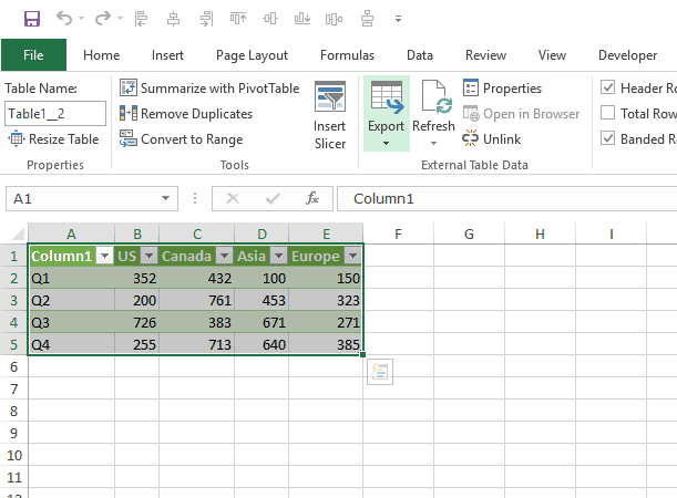
Suppose you have a dataset as shown below:

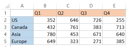
This data has the regions in a column and quarters in a row.

Now for some reason, if you need to transpose this data, here is how you can do this using paste special:

• Select the data set (in this case A1:E5).
• Copy the dataset (Control + C) or right-click and select copy.
• Now you can paste the transposed data in a new location. In this example, I want to copy in G1:K5, so right-click on cell G1 and select paste special.
• In the paste special dialogue box, check the transpose option in the bottom right.
• Click OK.

This would instantly copy and paste the data but in such a way that it has been transposed. Below is a demo showing the entire process.

The steps shown above copies the value, the formula (if any), as well as the format. If you only want to copy the value, select ‘value’ in the paste special dialog box.

Note that the copied data is static, and if you make any changes in the original data set, those changes would not be reflected in the transposed data.

If you want these transposed cells to be linked to the original cells, you can combine the power of Find & Replace with Paste Special.

Also read: How to Move Columns in Excel

Transpose Data using Paste Special and Find & Replace

Using Paste Special alone gives you static data. This means that if your original data changes and you want the transposed data to be updated as well, then you need to use Paste Special again to transpose it.

Here is a cool trick you can use to transpose the data and still have it linked with the original cells.

Suppose you have a dataset as shown below:

Here are the steps to transpose the data but keep the links intact:

• Select the data set (A1:E5).
• Copy it (Control + C, or right-click and select copy).
• Now you can paste the transposed data in a new location. In this example, I want to copy in G1:K5, so right-click on cell G1 and select paste special.
• In the Paste Special dialog box, click on the Paste Link button. This will give you the same data set, but here the cells are linked to the original data set (for example G1 is linked to A1, and G2 is linked to A2, and so on).
• With this new copied data selected, Press Control + H (or go to Home –> Editing –> Find & Select –> Replace). This will open the Find & Replace dialog box.
• In the Find & Replace dialog box, use the following:
  • In Find what: =
  • In Replace with: !@# (note that I am using !@# as it’s a unique combination of characters that is unlikely to be a part of your data. You can use any such unique set of characters).
• Click on Replace All. This will replace the equal to from the formula and you will have !@# followed by the cell reference in each cell.
• Right-click and copy the data set (or use Control + C).
• Select a new location, right-click and select paste special. In this example, I am pasting it in cell G7. You can paste it anywhere you want.
• In the Paste Special dialog box, select Transpose and click OK.
• Copy paste this newly created transposed data to the one from which it is created.
• Now open the Find and Replace dialog box again and replace !@# with =.

This will give you a linked data that has been transposed. If you make any changes in the original data set, the transposed data would automatically update.

Note: Since our original data has A1 as empty, you would need to manually delete the 0 in G1. The 0 appears when we paste links, as a link to an empty cell would still return a 0. Also, you’d need to format the new dataset (you can simply copy paste the format only from the original dataset).

Also read: Combine Two Cells in Excel

Transpose Data using Excel TRANSPOSE Function

Excel TRANSPOSE function – as the name suggests – can be used to transpose data in Excel.

Suppose you have a dataset as shown below:

Here are the steps to transpose it:

• Select the cells where you want to transpose the dataset. Note that you need to select the exact number of cells as the original data. So for example, if you have 2 rows and 3 columns, you need to select 3 rows and 2 columns of cells where you want the transposed data. In this case, since there are 5 rows and 5 columns, you need to select 5 rows and 5 columns.
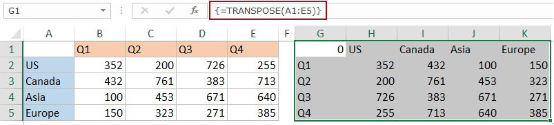
• Enter =TRANSPOSE(A1:E5) in the active cell (which should be the top left cell of the selection and press Control Shift Enter.

This would transpose the dataset.

Here are a few things you need to know about the TRANSPOSE function:

• It is an array function, so you need to use Control-Shift-Enter and not just Enter.
• You can not delete a part of the result. You need to delete the entire array of values that the TRANSPOSE function returns.
• Transpose function only copies the values, not the formatting.

Transpose Data Using Power Query

Power Query is a powerful tool that enables you to quickly transpose data in Excel.

Power Query is a part of Excel 2016 (Get & Transform in the Data tab) but if you’re using Excel 2013 or 2010, then you need to install it as an add-in.

Suppose you have the data set as shown below:

Here are the steps to transpose this data using Power Query:

In Excel 2016

• Select the data and go to Data –> Get & Transform –> From Table.
• In the Create Table dialogue box, make sure the range is correct and click OK. This will open the Query Editor dialog box.
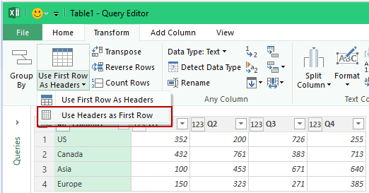
• In the Query editor dialog box, select the ‘Transform’ tab.
• In the Transform tab, go to Table –> Use First Row as Headers –> Use Headers as First Row. This ensures that the first row (that contains headers: Q1, Q2, Q3, and Q4) are also treated as data and transposed.
• Click on Transpose. This would instantly transpose the data.
• Click on Use First Row as Headers. This would now make the first row of the transposed data as headers.
• Go to File –> Close and Load. This will close the Power Editor window and create a new sheet that contains the transposed data.

Note that since the top left cell of our data set was empty, it gets a generic name Column1 (as shown below). You can delete this cell from the transposed data.

In Excel 2013/2010

In Excel 2013/10, you need to install Power Query as an add-in.

Click here to download the plugin and get installation instructions.

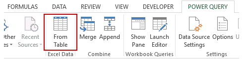
Once you have installed Power Query, go to Power Query –> Excel Data –> From Table.

This will open the create table dialog box. Now follow the same steps as shown for Excel 2016.

You May Also Like the Following Excel Tutorials:

• Multiply in Excel using Paste Special.
• CONCATENATE Excel Range (with and without separator).
• Clean Data in Excel Spreadsheets.
• Compare Columns in Excel
• Excel Text to Columns
• Excel TRIM Function
• Merge Tables in Excel